Performance evaluation of self-reconfigurable service ... - CiteSeerX

Performance evaluation of self-recongurable service-oriented software with stochastic Petri nets! Diego Perez-Palacin, Jos´e Merseguer Dpto. de Inform´atica e Ingenier´ıa de Sistemas, Universidad de Zaragoza, Zaragoza, Spain

Abstract Open-world software is a paradigm which allows to develop distributed and heterogeneous software systems. They can be built by integrating already developed third-party services, which use to declare QoS values (e.g., related to performance). It is true that these QoS values are subject to some uncertainties. Consequently, the performance of the systems using these services may unexpectedly decrease. A challenge for this kind of software is to self-adapt its behavior as a response to changes in the availability or performance of the required services. In this paper, we develop an approach to model self-rencongurable open-world software systems with stochastic Petri nets. Moreover, we develop strategies for a system to gain a new state where it can recover its availability or even improve its performance. Through an example, we apply these strategies and evaluate them to discover suitable recongurations for the system. Results will announce appropriate strategies for system performance enhancement.

1. Introduction In the new and exciting open-world software paradigm [1], the environment changes continuously and the software must dynamically react and adapt its behavior. The world is open to new components that the environment can dynamically provide and the software discover and bind. So, in an open-world, software is no longer created from scratch but integrating already developed third-party services. Currently, there exist approaches, standards and technologies partially supporting open-world software assumptions, among them, publish-subscribe middleware, grid computing, autonomic computing or service oriented architectures (SOA) [2, 3] and their underlying implementations such as web services. In this context, software services [4] are abstractions that should be exible enough to mix technologies (e.g., sensors, GPS or tag-based [5]), to execute in open environments (usually connected through networks) or to interplay without authorities. Finally, they are committed to provide adequate quality of service (QoS). ! This work has been supported by the project DPI2006-15390 of the Spanish Ministry of Science and Technology. Email addresses: [email protected] (Diego Perez-Palacin), [email protected] (Jos´e Merseguer)

Preprint submitted to Elsevier

September 1, 2009

Open-world software distinguishes the roles of service provider and service integrator. The former develops and deploys, probably in heterogeneous environments, services to be executed in unforeseen manners, and the latter creates service-based applications invoking those external deployed services. Service integration needs, among others, that deployed services: describe their functional and non-functional properties; provide and negotiate QoS levels (SLA); can be dynamically discovered and bound at runtime; allow their real behavior to be monitored. This paper mainly deals with the last two topics. Regarding the rst topic of interest, the fact that services can be discovered and bound at runtime means that service-based applications can change their internals to take advantage of recently deployed services. Therefore, services can change their current conguration, so they are considered as a kind of self-adaptive software [6]. Reconguration may take two forms: mandatory and optional. Mandatory reconfiguration occurs when the application cannot longer work with the current conguration. For example due to the disruption of the requested service or a failure in it. Garlan et al. dened a similar concept, self-healing systems [7]. Optional reconfiguration is used to improve system QoS, so although the system really still works, a reconguration will offer advantages such as better performance. Regarding the second topic, monitoring is also in the research agenda of the open-world software. The challenge here is to collect and analyze data from providers to be compared with the promised QoS (e.g., SLA in some technologies), check deviations and consequently plan strategies to react and recongure the system. Service integrators (humans and programs) should easily access the QoS parameters, dening the software services, to guide optional reconguration for improving system QoS. For instance, in SOA these parameters are called policies [8] and web services could declare them in the UDDI register. However, we and other researchers [9] make the point that this information could not be precise or updated or it could be even incorrect. So, our point is that the choice of provider, for a given service request, should be aware of the performance exhibited by all providers currently offering the service. When a system under development wants to incorporate this performance-aware reconguration property, an off-line approach can be taken to study its feasibility and to gain insight into possible reconfiguration strategies that eventually could be implemented to accomplish the property successfully. In this paper, we align with this off-line approach, then our system design will reect not only the workow of the service integrator, but also the reconguration strategies of interest and a “simulation” of the monitoring. From the software design, we will get a formal model, in terms of Petri nets, that will be evaluated to learn about the effectiveness of the reconguration strategies for this design. We recognize that the reconguration choice should consider not only performance but also other QoS attributes such as cost, reliability or security. So, the reader should understand that the conclusions we will obtain here will provide just a parameter for this nal reconguration choice. The balance of the paper is as follows. Section 2 describes the software design of the system under study. Section 3 evaluates gures for this system when only mandatory reconguration affects. Section 4 introduces optional reconguration and then the evaluation of different strategies makes sense. Finally, Section 5 revises the related work and gives a conclusion. 2

{PAoccurrencePattern= (’poisson’,0.005,’tu’)}



[Indoor] Internal Pre!process

lostWLAN

Call C2::S2 Internal Post!process

[Outdoor] Call C3::S2

{PAdemand=(’assm’, ’mean’,(3.5,’tu’))}

(a)

PAextOp=(C2_S2,1), PAdemand=(’assm’,’mean’,(10,’tu’))}

{PAextOp=(WLAN_transmit,1), PAdemand=(’assm’,’mean’,(1,’tu’))}

{PAextOp=(satellite_transmmit,1), PAdemand=(’assm’,’mean’,(3.5,’tu’))}

Indoor

(b) {PAextOp=(C3_S2,1), PAdemand=(’assm’,’mean’,(25,’tu’))}

Outdoor

getWLAN {PAdemand=(’assm’, ’mean’,(5,’tu’))}

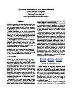
Figure 1: (a) Workow (b) Mandatory reconguration WLAN_NETWORK



S1

Host2

C1

C2

C1

S2

Application

C2



C3

Host3



C3

INTERNET

(b)

(a)

Figure 2: UML component and deployment diagrams

2. The system under study Component-based software engineering [10] (CBSE) is today a eld with wellestablished component models and technologies, for example, the Commercial Off The Shelf (COTS) components. Let us assume we need to develop a COTS component C1 to be assembled in applications for PDAs; it will offer one service or interface S1, see Figure 2 (a). According to the workow description in Figure 1(a), it happens that C1 needs to invoke the service S2 to properly carry out its duties. S2 is an already deployed service by C3 for eventual users in an open-world software context and it may also be provided by C2, see Figure 2 (a), being both C2 and C3 third party components. Therefore, the C1 component developer will not play the service provider role, since S1 will not be globally accessed, but s/he has to play as a service integrator selecting the proper provider (C2 or C3). The choice should consider the differences among these components, which actually account for service times and coverage. We may assume that C2 provides faster mean service time but smaller coverage since it can only be accessed from the wireless interface of the Local Area Network (LAN) where it executes, see deployment in Figure 2 (b). However, C3 offers the service through Internet via satellite, which can make it slower but specially suited for PDA users,

3

and moreover it provides global coverage for S2. Actually our example is inspired by the one in [11], so we will refer to this last situation as the outdoor configuration, while indoor configuration will refer to the PDA executing in LAN, say inside the University campus. We have also borrowed the state machine in Figure 1(b) from [11] to represent these possible congurations, changes among congurations are triggered by lostWLAN and getWLAN events the PDA should notify. Since C1 is under development, we aim to assess the performance S1 could offer. C1 will behave as a self-adaptive software, i.e., it decides self-reconfigurations to request S2 to the current best provider (say component). We will study two reconguration cases. The rst one, described by the workow and state machine in Figures 1(a,b), will be elaborated in Section 3. This is a case of mandatory reconfiguration since C1 changes from outdoor to indoor and vice-versa depending on the PDA location, but without the service integrator choice. The second reconguration case will be developed in Section 4 and it introduces a slight but very important change: when C1 is outdoor and it has to request S2, then it will be allowed to choose among C3 or C4, hence, optional reconfiguration is considered. The C3 or C4 choice will be based on a performance criteria. The component and deployment diagrams are shown in Figure 7(a) and 7(b), respectively. The workow and state machine are given in Figure 8(a) and 8(b). Workload WorkloadType=’open’ ArrivalProcess=0.005

from to

ServiceCall

Start from

Resource type="C1" name="C1" capacity=1 scheduling="FIFO"

to

Activity name="InternalPreProcess" internalExecTime=3.5

Service name="S1" Behavior

from to

Activity

from to

offered Service

name="Call_S2" resourceType="S2_server" serviceName="S2" isSynch=true

ServiceCall name="transmission" resourceType="net" serviceName="transmit" isSynch=true

name="InternalPostProcess" internalExecTime=5 from to

End

Figure 3: Klaper model of the workow

System performance view The system performance characteristics have been annotated with the standard UML prole for Schedulability, Performance and Time Specication (SPT) [12]. The workow in Figure 1(a) describes some performance parameters. Here, execution demands for S1 internal activities are 3.5 and 5 time units respectively. Besides, an S2 call implies two external operations and their corresponding demands (WLAN and C2::S2

4

or satellite and C3::S2). As previously suggested, the way to get these values will depend on the technology. Resource type="C2" name="C2" capacity=* scheduling="FIFO"

Resource type="OpenWorldInterface" name="OpenWorld" capacity=* scheduling="FIFO" offered Service Service

offered Service Service name="S2"

name="S2_interface" Behavior

Behavior

Resource type="C3" name="C3" capacity=* scheduling="FIFO"

offered Service

Resource type="net" name="net" capacity=* scheduling="FIFO" offered Service

offered Service Service name="S2"

Service name= "satellite" Behavior

Service name= "wireless" Behavior

Behavior Start

Start

from

from

Activity name="C2_S2" intExecTime=10 from

End

Start

(a)

from

to

End

to

(b)

Activity name="C3_S2" intExecTime=25

End

to

Activity

intExecTime=3.5 name= "WLAN_transmit"

from to

from

Activity

to

name="Call_S2" ResourceType="S2_server" ServiceName="S2" isSynch=true

Start

from

from

to

ServiceCall

to

to

Start

(c)

intExecTime=1.0 name= "satellite_transmit"

from

from to

End

(d)

to

End

Figure 4: Klaper model of the resources

So far we have proposed a UML-SPT design that describes the system and its performance characteristics. From this software design different performance models could be obtained (e.g., queuing networks, stochastic Petri nets or stochastic process algebras) following the proposals in the literature, some of them surveyed in [13]. However, we prefer to convert the design into a D-Klaper [11] model since it brings some advantages. Moreover, there exists an automatic model-transformation [11] from UML-SPT to D-Klaper (which justies why we currently use SPT instead of the more recent MARTE [14] prole). Later, we will gain a performance model from D-Klaper, indeed D-Klaper is a suitable intermediate model that helps to bridge the gap between UML-SPT designs and different performance models. Figures 3, 4, 5 (a,d) and 6 span the D-Klaper obtained for both designs, mandatory and optional. D-Klaper explicitly describes the bindings, which are important to understand system recongurations; here we assumed they do not consume time. Moreover, it also makes explicit the use of services and resources as well as their performance characteristics. Among the latter, D-Klaper describes the capacity of resources, which in this case are not restricted (so, they are all set to *, see Figure 4), then accounting for the fact that C2 and C3 may serve other requests from other components. Although there does not exist yet an automatic model-transformation from D-Klaper to Petri nets, we can manually obtain the net (later outlined). Moreover a brief discussion around how to bridge the semantic gap between D-Klaper and Petri nets through an automatic translation will be given in the Conclusion. The major drawback of D-Klaper, from our point of view, is that it can not deal with the received events in UML state machines. However we had to translate a number of them into D-Klaper (Figure 5), our solution has been to introduce 5

a ReceiveEvent model element (see grey boxes in Figure 5) that accounts for the received events in a UML state machine. Behavior

Workload population=1

Start

Workload population=1

Workload population=1

Workload population=1

from to

Activity name="Indoor" 3 internalExecTime= 10

Resource type="Monitor" name="Monitor" capacity=1 scheduling=FIFO

to

from to

DestroyBinding name=outWLAN sourceStep=C1.S1.transmission targetService=net.wireless

Resource type="CurrConfig" name="CurrConfig" capacity=1 scheduling=FIFO

Resource type="ReconfStrategy" name="ReconfStrategy" capacity=1 scheduling=FIFO

Service name="Monitoring"

Service name="Config"

Service name="RunStrategy"

from

Behavior

to

DestroyBinding name=outC2 sourceStep=C1.S1.Call_S2 targetService=C2.S2 from

Start

to

CreateBinding name=inSatellite sourceStep=C1.S1.transmission targetService=net.satellite

Activity name="Idle" internalExecTime=0.0

from

from

from to

DestroyBinding name=outOpenWorld sourceStep=C1.S1.Call_S2 targetService=OpenWorld.S2_interface from

to

from

DestroyBinding name=outC3 sourceStep=OpenWorld. S2_interface.CallS2 targetService=C3.S2

from to

to

ServiceCall name="toActivateC4" resourceType="CurrConfig" serviceName="Config" name="ActivateC4" isSynch=false

Activity name="MoreThan" " internalExecTime=0.0 ReceiveEvent name="Response"

from

to

ServiceCall name="notificationSlow" resourceType="ReconfStrategy" serviceName="RunStrategy" name="Slow" isSynch=false ReceiveEvent name="Response" from to

from to

CreateBinding name=inC4 sourceStep=OpenWorld. S2_interface.CallS2 targetService=C4.S2

to

from

Activity name="ReqC4" internalExecTime=!

from

from

ReceiveEvent name="ActivateC3" from

to

ServiceCall name="toActivateC3" resourceType="CurrConfig" serviceName="Config" name="ActivateC3" isSynch=false

to

DestroyBinding name=outC3 sourceStep=OpenWorld. S2_interface.CallS2 targetService=C4.S2 from to

from

(c)

(b)

from

CreateBinding name=inC4 sourceStep=OpenWorld. S2_interface.CallS2 targetService=C3.S2

ServiceCall name="notificationSlow" resourceType="ReconfStrategy" serviceName="RunStrategy" name="OK" isSynch=false

(a)

to

ReceiveEvent name="ActivateC4"

ReceiveEvent name="OK"

ReceiveEvent name="Slow"

from

from

to

Activity name="UsingC3" internalExecTime=0.0

to

Activity name="LessThan "" internalExecTime= "

from

CreateBinding name=inC2 sourceStep=C1.S1.Call_S2 targetService=C2.S2

to

from to

to

CreateBinding name=inWLAN sourceStep=C1.S1.transmission targetService=net.wireless

to

from

to

DestroyBinding name=outSatellite sourceStep=C1.S1.transmission targetService=net.satellite

Activity name="0!Slow" internalExecTime=0.0 to

to

Activity name="Outdoor" 3 internalExecTime= 2 · 10

to

to

ReceiveEvent name="Request"

to

from

from

from to

from

CreateBinding name=inOpenWorld sourceStep=C1.S1.Call_S2 targetService=OpenWorld.S2_interface

Start

Start

from to

Behavior

Behavior

(d)

Figure 5: Klaper models: (a) mandatory reconguration in Fig. 1 (b), (b) monitor in Fig. 10, (c) strategy in Fig. 11(b), (d) optional reconguration in Fig. 8 (b)

3. Self-healing reconfiguration This section focusses on the performance evaluation of the system already presented when mandatory reconfiguration applies. Actually, this reconguration acts as a self-healing process [7], because when the system changes from indoor to outdoor, the current request to C2::S2 is lost and the system damaged due to unavailability. Then, a repair or reconguration is mandatory. However, when the change is from outdoor to indoor, although the system may still work, we carry out a reconguration 6

assuming that a LAN connection may be for free or at least cheaper than a satellite connection. The performance evaluation will be carried out using the Petri net in Figure 13 (a), that has been manually created from the D-Klaper model. We have emphasized different subnets within dotted frameworks. The subnet on the left models C1::S1 workow, it comes from Figure 3. The four subnets in the middle represent the resources required by S1, they come from Figure 4. The last subnet models the conguration in use and the reconguration actions and comes from Figure 5 (a). This Petri net is a Generalized Stochastic Petri Net [15] (GSPN) and it accounts for all possible systems congurations (indoor or outdoor). Let us discuss some technical details regarding the GSPN in Figure 13 (a). The time modeled in D-Klaper for each activity is represented in the GSPN either by an exponential transition with mean ring time equal to internalExecTime or by an immediate one depending on whether that value is greater than zero or not. It is important to remember that D-Klaper does not consider events, in this case we represent getWLAN and lostWLAN (Figure 1(b)) as D-Klaper timed activities (indoor and outdoor in Figure 5) instead of using the proposed ReceiveEvent. In this case this is feasible since we can assume that the system will spend an amount of time in indoor and an amount in outdoor, therefore the events can be written off. The time spent by these activities has been set to 103 and 2 · 103 respectively, therefore we are evaluating a system that spends twice as much time outdoor as indoor. In the GSPN, these activities are represented by transitions T40|indoor and T45|outdoor, concretely in the Reconfiguration subnet. Finally, we remark that in the subnet C1::S1, P 18 models a decision since it enables t21 or t24 depending on the conguration (indoor or outdoor), also in this subnet, t37 and t39 are responsible for the operations interruption when the system changes from indoor to outdoor. In this case, execution returns to P 17 and the service calls will be re-launched to C3. Petri net evaluation results Result Mean response time Mean utilization

Mean throughput % of interrupted re-

C1::S1 C1 C2 C3 WLAN Satellite C2::S2 C3::S2 WLAN

35.8 0.138 0.016619 0.0833944 0.0016634 0.0116882 0.00166 0.00333 0.01

quests C2::S2 0.1 χt is the mean throughput of transition t #P is the mean number of tokens of place P

Formula 1−#P17+#P5 χT1

1 − #P17 #P3 #P4 #P1 #P2 χt29 χt31 χt37 · 100 χt21 χt39 · 100 χt28

Table 1: Results of the mandatory or self-healing reconguration

7

We are interested in evaluating the GSPN to get performance gures when the system alternates indoor and outdoor. Table 1 gives the results, which were obtained with the GreatSPN tool [16] simulation programs. The most interesting result, from the service integrator point of view, would be S1 response time, 35.8 t.u., now s/he should check if this result fullls the requirements. Concerning the mean C2, C3, LAN and satellite utilizations, they seem very low, though these values refer only their use by C1, but actually they will be used by other open world components, so the providers are responsible for guaranteeing their mean response times (10 and 25 t.u. for C2 and C3 respectively). Same comment applies to mean throughput rows, that in this case obviously relates the number of requests processed by C2::S2 with respect to C3::S2. Finally, the percentage of interrupted requests means those requests not completed due to a change in the conguration. It only applies to indoor→outdoor changes, and both the WLAN and the waiting for C2::S2 can be affected. 4. Optional reconfiguration

Resource type="C3" name="C3" capacity=* scheduling="FIFO" offered Service Service name="S2" Behavior

Start

from

Activity name="servS2" intExecTime=10 to

End

Behavior

Start

from to

from

Resource type="C4" name="C4" capacity=* scheduling="FIFO"

Start

to

from

Activity name="servS2" intExecTime=70 from

offered Service Service name="S2" Behavior

to

(a)

End

to

Activity name="servS2" internalExecTime=35 from to

End

(b)

Figure 6: Klaper model: (a) C3::S2 (b) C4::S2

Now, we focus our study in the same system but introducing optional reconfiguration with the aim of improving performance in C1::S1. The system design depicted in Figures 7 and 8, allows C1 in outdoor configuration to choose the better performing component among C3 and C4. Performance specification Consider that the QoS specication in C3 still declares for S2 a mean response time of 25 time units while C4 QoS declares 35, both exponentially distributed. The workow in Figure 8 (a) depicts these values, annotations already given in Figure 1(a)

8

have been omitted. Now, let us distrust the C3 QoS declaration, then we decide to monitor this component to get more accurate gures about its real behavior. Finally, we realize that C3::S2 works in two differentiated modes: peak hours mode, which in mean lasts for six hours per day and exhibits an exponentially distributed response time with mean 70 time units; and normal mode, rest of the day, being its mean response time only 10 time units. Although C3 functional behavior is still a black-box, we could detail its monitored performance behavior, see the subnet in Figure 9 (b). Transitions T1, T2, T3 and T4 are exponentially distributed with means respectively x, y, 70 and 10. Since T1 and T2 respectively model the time spent in peak hours and normal modes then x needs to be three times slower than y (6 and 18 hours respectively). Actually, this net preserves a mean time of 25 time units as declared in Figure 8(a) for C3::S2, therefore the QoS declaration for C3 was correct; in fact our suspicions arose from this high variability among peak and normal.

WLAN_NETWORK

Host2 C2

S1



C1 S2



Host3

C1

C3



C2

C3

C4

Application



(a)

INTERNET

(b)

Host4 C4

Figure 7: UML component and deployment diagrams

Let us present the aim of the study. From Figure 8 (a), we may naively infer that being the mean response time 25 in C3 and 35 in C4, then the service integrator choice should always address C3, hence reducing the problem to the one in previous section. This would be true only if whatever two consecutive requests to C3 were always independent, as requests to C4 are. However, since C3 owns these two well-known different operation modes, we positively know that requests are not independent, so they have to belong to one mode or the other. Therefore, as long as the service time values obtained in the most recent requests to C3 were available, then it would be possible to predict the mean service time for the following requests to C3. This would be true if we assume that the predicted requests will belong to the same C3 operation mode as the ones already tracked. Remember that we got precise gures for these modes (10 and 70 t.u.), and we can apply them in the prediction. Hence, S1 performance may be improved if we are able to address the current request to S2 to the component (C3 or C4) currently working at the lowest estimated response time, i.e., to address C4 (35 t.u.) when C3 is 9

Internal Pre!process

[Using C3]

[Indoor] [Outdoor]

[Using C4]

PAdemand=(’assm’,’mean’,(25,’tu’))}

Call C3::S2

PAdemand=(’assm’,’mean’,(35,’tu’))}

Call C4::S2

activateC4

Call C2::S2 Internal Post!process

PAdemand=(’assm’,’mean’,(10,’tu’))}

UsingC3

(a)

(b)

UsingC4

activateC3

Figure 8: (a) Workow (b) Optional reconguration request request

C3::S2 T1|x

C3::S2

T2|y

T3|C3_S2 T4|C3_S2 response response

(a)

(b)

Figure 9: Detailed performance behavior in C3::S2

in peak hours (70 t.u) or to address C3 when it works in normal mode (10 t.u.). From the previous two paragraphs we can conclude that it would be very interesting for an open-world component to be equipped with monitors that keep track of those untrusted services it uses. So, the monitor could get accurate figures describing these services. Besides, it would be of interest that another module could take advantage from the monitored information by implementing strategies able to predict for each request the provider that currently could offer better service. In the following, we discuss the implications of such monitor and reconfiguration strategies in our UML design and Petri net. 4.1. Service monitoring and reconfiguration strategies The UML design of the monitor in Figure 10 (a) is a state machine that is initially idle and it is activated when a request is sent to the tracked component, and then waits for the component response. If the time spent between these two calls is smaller that τ the correct behavior is notied to the system (okC3) otherwise an alarm about the malfunction is raised (slowC3). The D-Klaper model corresponding to the monitor appears in Figure 5(b). From the D-Klaper we will get a subnet (Figure 10 (b)) 10

that can be seen as a black-box module with well-dened interfaces (Figure 10(c)). The input interfaces account for the calls (requestC3 and responseC3) addressed to the provider who is being tracked. The outputs (slowC3 or okC3) will inform about the provider’s performance. These places (inputs and outputs) will be merged, in the system Petri net in Figure 13(b), to their peers with equal name. Then the monitor will be aware of the actual requests and responses. Consider that there will be in the system Petri net as many identical black-box monitor modules as providers we need to track, in our case only one, C3. Finally, it is worth noting that the monitor subnet (Figure 10 (b)) does not inuence the performance in the rest of the net. t1|requestC3

t3|responseC3 requestC3 responseC3

requestC3 Idle

Idle

LessThan " responseC3/okC3

responseC3/slowC3

MoreThan"

LessThan t

T2

MONITOR

"

After( ") MoreThan t

P6|okC3

(a)

P5|slowC3

(b)

okC3

slowC3

(c)

Figure 10: Monitor module

Reconfiguration strategies aim to select, assisted by the monitor, the current best provider regarding performance. They will also be modeled as a black-box module, that we will call reconfiguration controller (Figure 11 (a)). In the UML design, we will represent each strategy with a state machine, although we are currently investigating more expressive approaches. We include in Figure 11 (b,d) two simple examples for this system, the D-Klaper model corresponding to the rst strategy appears in Figure 5 (c). This rst strategy recongures the system the very rst time the monitor detects the provider is working slowly, while the second strategy needs two consecutive slowC3 events from the monitor to carry out reconguration. So, the events in transitions (e.g., slowC3 in Figure 11 (b)) are received from the monitor module, and they can trigger another event (e.g., activateC4 is the one triggered in slowC3/activateC4). activateC4 is sent to the state machine in Figure 8 (b) to actually change the current system conguration. On the other hand, the change from C4 to C3 is accomplished in both strategies when expires a given time, say λ (Figure 11 (b,d)). Figure 5(c) depicts the D-Klaper models of the strategies, they will be converted into reconfiguration controller subnets (Figure 11(c,e)). The reconfiguration controller input interfaces (Figure 11 (a)) are the monitors outputs, which in fact are the events the strategy needs to work (okC3 and slowC3). The output interfaces provoke the system reconguration as discussed in the previous paragraph for activateC4. Again these interfaces will be merged with the places, in the system Petri net, with equal names. As a result, the monitor and the reconfiguration controller will cooperate. Note that we can get as many system Petri nets as reconfiguration controller modules we dene. Hence, a system Petri net represents the system with a given reconguration

11

okC3 slowC3

okCn slowCn .........

RECONFIGURATION CONTROLLER ......... activateC3 okC3

(a)

activateCn okC3

slowC3

okC3

slowC3

okC3 0!slowC3 reqC3

0!slowC3 reqC4

1!slowC3

reqC3 okC3

slowC3/activateC4

!

slowC3

1!slowC3

slowC3/activateC4

reqC4

After (!)/activateC3

reqC4 !

After (!) /activateC3

reqC4 activateC4

activateC4 activateC3

(b)

(d)

(c)

activateC3

(e)

Figure 11: Reconguration strategies

strategy. Figure 13 (b) shows the Petri net that models the whole system. An important difference with the one corresponding to the previous section, Figure 13 (a), is that now it belongs to the Deterministic Stochastic Petri Net [17] (DSPN) class instead of GSPN. The reason is that monitor’s T2 transition is deterministic instead of exponentially distributed. As a conclusion, we have obtained a Petri net (Figure 13 (b)) by translating the DKlaper models. This net will be used for evaluation and it models the system workow, the components that need special tracking, the strategy for reconguration and the monitor. 4.2. System evaluation results The obtained Petri net will be useful for service integrators to assess performance characteristics of the system, e.g., to verify that S1 meets the required response time or to suggest which components should be changed or improved to accomplish this target. In this section, we will use the Petri net in Figure 13 (b) for another purpose of interest, the evaluation and comparison of the proposed reconfiguration strategies. From this study, we will discover which ones perform better or reach a necessary performance threshold. Consider that in a real situation, the service integrator will be interested in a few strategies, those actually making sense in the problem domain. In particular, we identied three scenarios of interest:

12

• Scenario one (s1) considers strategy in Figure 11 (b): In this case the monitor will send the event slowC3 when detects a request exceeding 35 time units. The reconfiguration controller module is the subnet in Figure 11 (c). • Scenario two (s2) considers strategy in Figure 11 (d): In this case the monitor will send the event slowC3 also when detects a request exceeding 35 time units. But in this case two consecutive events are needed for the controller to recongure. The controller module is the subnet in Figure 11 (e). • Scenario three (s3) considers strategy in Figure 11 (b): However in this case the monitor will send the event slowC3 when detects a request exceeding 70 time units. Again , the reconfiguration controller module is the one in Figure 11 (c). The values selected for these scenarios are not arbitrary ones. In fact, we have carried out lots of evaluations of the net (with different values) to nally realize that these ones actually represent strategies of interest. s1 matches with an “impatient” service integrator who changes conguration without “strong reasons”. Scenarios s2 and s3 wait for more “real reasons” to change system conguration. Additionally, we also consider the following scenarios, they will help us to realize the actual performance improvements among the previous ones. • Scenario four (sect3): all the Outdoor requests address C3. In fact, this is the scenario carried out in Section 3. • Scenario ve (random): applies a random selection among C3 and C4 (with probability 0.5 for each one). • Scenario six (ideal): assuming that the system knows for each request which component performs better. Obviously this would be impracticable in a real system, since the only way to know the current response time is to perform the real request. Once we settled these six scenarios, we dened four experiments to accomplish our goal. The results in experiment (a.1) were computed using the formula in the rst row in Table 1, but obviously applied to the Petri net in Figure 13 (b). The results in experiment (d), were computed also in the Petri net in Figure 13(b), later explained. On the other hand, (b,c) were computed in terms of the probability to reach M " from M . For example, in the case of (b), M is the set of markings that in the domain can be interpreted as the system using C3 and C3 working in normal mode, while M " represents the use of C4 being C3 in normal mode. We avoid to give a formal denition of M and M " in terms of the Petri Net due to lack of space. We also note that in the case of the ideal scenario, the Petri net in Figure 13 (b) had to be slightly modied since it had to test if C3 was in normal mode to address the request. The rst experiment, in Figure 12 (a.1), was to compute the mean response time (RT) achieved by S1, which actually means to compare the effectiveness of the strategies. The graph obviously pointed out ideal as the best and random as the worst. The reconguration strategies (s1, s2, s3) seem to offer similar results. However, in Figure 12 (a.2) we show that the “relative” improvement among them is signicant. We 13

Figure 12: Optional reconfiguration evaluation results

say “relative” because we consider that the best RT they could achieve is the one given by ideal. So, we have “normalized” these values w.r.t. ideal. The second experiment is depicted in graph (b). It shows what we call “wrong recongurations”, i.e., the situation where C3 is working in normal mode but the strategy wrongly predicts that C3 has changed to peak hours mode, so the strategy wrongly decides to start invoking C4. Note that there not exist “wrong recongurations” for C4, because the strategy changes from C4 to C3 just when a given λ time has elapsed. The results in (b) again conrm our intuition: the worst strategy is the one that changes the current conguration without “strong reasons”. In our example, it means that s1 changes to C4 the very rst time a response time greater than 35 is obtained from C3. However, the other two strategies perform very few “wrong recongurations”, they change only when “there are real reasons” (two C3 response time greater than 35 or one greater than 70). The third experiment, in Figure 12 (c), aims to discover the percentage of S2 requests actually addressing the potentially faster component in every moment. In short, the requests that address C3 when it works in normal mode and address C4 when C3 is in peak hours, we call it “hit rate”. Although being s2 and s3 the best strategies, they do not outperform s1 by far. However, in the second experiment, s1 showed a large number of “wrong recongurations”. Then, why s1 is not giving a signicant worse “hit rate” than the others?. In fact, these last two experiments do not show the number of “necessary recongurations” that neither s2 nor s3 carry out, but s1 does. The next experiment may give a light in this regard. The fourth and last experiment, Figure 12 (d), investigates the “reconguration rate” in our three strategies. “Reconguration rate” means the mean number of recongurations that are carried out during 100 executions of S1. In the Petri net we computed it as χχt50 T1 · 100. We observe that s1 performs more recongurations than the others. Actually, some of these recongurations are “wrong”, but the others “necessary”. In the case of s1, this explains that its large number of “wrong recongurations” is balanced with the “necessary” ones to nally get a “hit rate” similar to the other strategies. In the case of s2 and s3, it is clear that from the recongurations they perform, a few were “wrong”.

14

The conclusion for our study could be as simple as to say that an appropriate reconguration strategy regarding performance would be s3, since it offers the best response time, the highest “hit rate” and a low number of “wrong recongurations”. However, the study offers elements to the service integrator to more accurately evaluate the strategies. For example, if the effort of the system to perform a reconguration has to be considered (e.g. in terms of power consumption), then the best reconguration policy would be s2, since although it offers a worse RT than s3, its “reconguration rate” is lower. 5. Conclusion and related work During the last years, there has been a growing concern about systems that may automatically take decisions regarding their own behavior. They are known as self-* systems [18] and deal with properties such as self-managing [19, 20], self-reconguration, self-adaptation [21] or self-healing [7]. We have learned about these systems from Laddaga [22, 23]. Moreover, this work spans other elds such as performance evaluation with Petri nets, open-world software or QoS improvement. From Ghezzi and colleagues [1, 4, 9] we learned the implications of the open-world software paradigm in performance evaluation. Concretely, we addressed in this work topics in the research agenda of this paradigm concerning service monitoring and the selection of strategies to recongure the system aiming to improve its performance. In this paper we have built on our experience in evaluating performance of webservices [24] technology. However, we have taken a new direction, that of open-world software, that can be seen as a paradigm integrating technologies around software services architectures. So, we have rstly modelled and evaluated with Petri nets the selfhealing reconfiguration problem, so far we do not know another similar work. Once we understood this problem, we targeted the modeling of optional reconfiguration aimed to improve system performance, then we realized the importance of monitoring the services and of exploring alternative strategies to predict for each request the better available service. Hence, nally the work focussed on modelling and comparing such strategies. As a result of this work, we consider that we have given a rst step towards a methodology for service integrators to automatically evaluate their service-oriented designs. Our approach produces a Petri net that models: the system functionality in terms of the service integrator’s workow; the detailed performance behavior of the services that need special tracking; the strategy for reconguration; and moreover this net embeds a monitor that keeps track of the current response times of these special services. This Petri net is useful for service integrators in different manners, such as: to assess system performance characteristics, to tune software designs considering QoS, to test different performance-aware reconguration strategies in the service composition. This paper has only explored the last one and throughout a limited number of scenarios in an easy to understand example. However the approach here developed could be applied to more complex systems, i.e. those with lots of possible congurations due to the existence of multiple and required services and a great amount of providers offering them. In this case, the approach will apply as many strategies as services are required, each strategy should manage one service and should predict its 15

best provider. On the other hand, this work could be seen as an extension of the one in [25] since it produces a unied model for service oriented designs that may embrace performance, reliability and reconguration. We would like to evaluate our proposal concerning some relevant aspects regarding the modeling of self-adaptable systems, the work of Geihs [26] points out some modeling concerns that have to be addressed: • All the service configurations have to be modeled. In our case, the workow described in the activity diagram spans this information, while the components and deployment diagrams depict which components offer the services and where are located. • Context dependencies that determine when and how a service reacts. The state machines describing the strategies embed this information. • Service-types and substitutability. The rst topic is represented in our component and deployment diagrams and the latter in the state machines for reconguration. • Adaptation reasoning to select the best configuration in a certain situation. This is accomplished by the reconguration strategies. • Non-functional service properties and requirements. We represent them using SPT annotations, although as discussed, MARTE would also help. However some complex properties, such us to associate different behaviors to the same service (e.g., with different QoS) cannot be annotated with these proles. • Architectural constraints for the service configuration and resource constraint and dependencies. These topics are not addressed in our proposal yet. Some other aspects of our approach deserve a detailed discussion. A rst topic concerns about the class of DSPN. This class arises in our approach when we introduce deterministic transitions in the monitor. So far it has been necessary to introduce only one deterministic transition, but a monitor could need more than one, in this case they should not be concurrently enabled if we desire to use exact analysis techniques to solve the DSPN. However, the DSPN could be always solved using simulation techniques even in the presence of multiple concurrently enabled deterministic transitions. Therefore, this DSPN characteristic is a real drawback only when exact analysis is used. A second topic is about D-Klaper. As we pointed out, it has not been designed to explicitly deal with events. However, our approach uses UML state machines and they trigger events. So, we have solved this problem introducing a new meta-class Event in the D-Klaper metamodel. However we consider that this fact should be subject of painstaking research in the D-Klaper context. A third topic considers lling the gap between D-Klaper and Petri nets. The works of Grassi et al. [27, 25, 11] describe transformations from Klaper to extended queuing networks, discrete time Markov processes and semi-Markov reward models (SMR), but not to Petri nets. These transformations are based on the Meta-Object Facility [28] (MOF) and apply MDA techniques that can be also valid for a Petri net transformation using for example the Petri net MOF dened in [29]. 16

As a future work we should consider among others the following issues: a set of monitors and a library of reconfiguration controllers, the latter implementing standard strategies and even parameterizing them; an automatic translation of the designs models into Petri nets as well as to automate the Petri net evaluation. Regarding the last two topics, we have gained some experience developing the ArgoSPE tool [30]. 5.1. Related work The works of Menasc´e [31, 32, 33, 34], although not focussed on the open-world paradigm, were fundamental to understand the model-based evaluation of servicebased applications, web-services and middleware in general. Menasce in [34, 33] uses brokers to negotiate and manage the QoS between clients requirements and services offered, at the same time different workloads can be managed. These works consider that the QoS values of the third-party providers are negotiated and hence well-known and reliable. However our work prefers not to blindly trust in such values but to track the providers to predict the current QoS, then our results would not be so precise. Indeed, our solution was inspired by the works [9, 22, 35]. Also in [36] is addressed the problem of guaranteeing the QoS of untrusted third-party services. They propose a framework to choose the better services in terms of QoS, but in contrast to our work the workload is balanced among several providers to support some kind of fault tolerance. [37] studies the problem of getting an optimal service composition not only in terms of performance but also of price and payload. Although our work currently considers performance only, it would be useful to introduce these other variables following the approach in [37], then getting the service integrator stronger arguments to select the service. The works of Grassi et al. [27, 25, 11] inuenced our approach by the adoption of their D-Klaper language, which is an intermediate model very well suited to represent core aspects of the service-based applications and recongurable systems, such as the binding among a service and its call. These features place D-Klaper as a better choice in this context than others such as the CSM [38, 39]. Klaper is also an asset to convert a UML design into a performance model. The SMR model obtained by Grassi in [11] splits to dene a reconfiguration model and as many performance models as congurations exits, which in our opinion penalizes the model analysis stage. However, the target performance model, i.e. Petri net, we get from D-Klaper accounts for all possible system congurations. The work in [40] studies policies to select appropriate servers, they consider the mean number of works and the mean service time and assume that the servers availability and reliability are well-known. In our work these assumptions do not hold since our servers are third party providers, then the most we can do is to track their response times. [41] researches policies to improve server allocation and stream admission decisions. The authors want to ensure servers QoS while improving revenues serving streams of requests. In this case improvements come from the server side, while in our work is the client who implements policies to improve the QoS.

17

References [1] L. Baresi, E. D. Nitto, C. Ghezzi, Toward open-world software: Issue and challenges, Computer 39 (10) (2006) 36–43. [2] M. P. Papazoglou, D. Georgakopoulos, Service-oriented computing, Communications of the ACM 46 (10) (2003) 25–28. [3] N. Josuttis, SOA in practice: The art of distributed systems design, O’Reilly, 2007. [4] E. D. Nitto, C. Ghezzi, A. Metzger, M. P. Papazoglou, K. Pohl, A journey to highly dynamic, selfadaptive service-based applications, Automated Software Engineering 15 (3-4) (2008) 313–341. [5] The Extensible Markup Language (XML), http://www.w3.org/XML. [6] DARPA, Self adaptive software, DARPA, BAA 98-12, Proposer Information Pamphlet (December 1997). [7] D. Garlan, J. Kramer, A. L. Wolf (Eds.), Proceedings of the First Workshop on Self-Healing Systems, WOSS 2002, Charleston, South Carolina, USA, November 18-19, 2002, ACM, 2002. [8] F. Curbera, Component contracts in service-oriented architectures, Computer 40 (11) (2007) 74–80. [9] L. Baresi, C. Ghezzi, S. Guinea, Smart monitors for composed services, in: ICSOC ’04: Proceedings of the 2nd international conference on Service oriented computing, ACM, New York, NY, USA, 2004, pp. 193–202. [10] I. Crnkovic, M. Larsson (Eds.), Building Reliable Component-Based Software Systems, Artech House, 2002. [11] V. Grassi, R. Mirandola, A. Sabetta, A model-driven approach to performability analysis of dynamically recongurable component-based systems, in: WOSP ’07: Proceedings of the 6th international workshop on Software and performance, ACM, New York, NY, USA, 2007, pp. 103–114. [12] OMG, UML Prole for Schedulability, Performance, and Time, version 1.1, formal/05-01-02 (January 2005). [13] S. Balsamo, A. D. Marco, P. Inverardi, M. Simeoni, Model-based performance prediction in software development: A survey, IEEE Transactions on Software Engineering 30 (5) (2004) 295–310. [14] Object Management Group, http://www.promarte.org, A UML Prole for MARTE (2005). [15] M. Ajmone Marsan, G. Balbo, G. Conte, S. Donatelli, G. Franceschinis, Modelling with Generalized Stochastic Petri Nets, John Wiley Series in Parallel Computing - Chichester, 1995. [16] The GreatSPN tool, http://www.di.unito.it/˜greatspn. [17] M. Ajmone Marsan, G. Chiola, On petri nets with deterministic and exponentially distributed ring times, in: Advances in Petri Nets 1987, covers the 7th European Workshop on Applications and Theory of Petri Nets, Springer-Verlag, London, UK, 1987, pp. 132–145. [18] O. Babaoglu, M. Jelasity, A. Montresor, C. Fetzer, S. Leonardi, A. van Moorsel, M. van Steen (Eds.), Self-Star Properties in Complex Information Systems, Vol. 3460 of LNCS, Hot Topics, SpringerVerlag, 2005. [19] D. Garlan, J. Kramer, A. L. Wolf (Eds.), Proceedings of the 1st ACM SIGSOFT Workshop on SelfManaged Systems, WOSS 2004, Newport Beach, California, USA, October 31 - November 1, 2004, ACM, 2004. [20] J. Kramer, J. Magee, Self-managed systems: an architectural challenge, in: FOSE ’07: 2007 Future of Software Engineering, IEEE Computer Society, Washington, DC, USA, 2007, pp. 259–268.

18

[21] R. Laddaga, P. Robertson, H. E. Shrobe (Eds.), Self-Adaptive Software, Second International Workshop, IWSAS 2001, Balatonf¨ured, Hungary, May 17-19, 2001 Revised Papers, Vol. 2614 of LNCS, Springer, 2003. [22] R. Laddaga, P. Robertson, Self adaptive software: A position paper, in: SELF-STAR: International Workshop on Self-* Properties in Complex Information Systems, 2004. [23] R. Laddaga, Active software, in: IWSAS, 2000, pp. 11–26. [24] E. G´omez-Mart´nez, J. Merseguer, Impact of SOAP implementations in the performance of a web service–based application, in: LNCS, Vol. 4331, Springer–Verlag, 2006, pp. 884–896. [25] V. Grassi, R. Mirandola, A. Sabetta, Filling the gap between design and performance/reliability models of component-based systems: A model-driven approach, Journal of Systems and Software 80 (4) (2007) 528–558. [26] K. Geihs, A development framework for adaptive pervasive applications, IEEE International Conference on Pervasive Services (2007) 332–334. [27] V. Grassi, R. Mirandola, A. Sabetta, From design to analysis models: a kernel language for performance and reliability analysis of component-based systems., in: Proceedings of the Fifth International Workshop on Software and Performance (WOSP’05), 2005, pp. 25–36. [28] Object Management Group, Meta Object Facility (MOF) Core Specication Version 2.0 (2006). [29] H. L. dos Santos, P. R. M. Maciel, N. S. Rosa, R. S. M. Barros, Managing Petri nets in MOF repositories., in: LNCS, 3761, Springer-Verlag, 2005, pp. 1381–1397. [30] E. G´omez Mart´nez, J. Merseguer, ArgoSPE: Model-based software performance engineering, in: 27th ICATPN, Vol. 4024 of LNCS, Springer, 2006, pp. 401–410. [31] D. Menasce, V. Almeida, Capacity planning for web services, Prentice Hall, 2002. [32] D. Menasce, Composing web services: a QoS view, IEEE Internet Computing 8 (6) (2004) 80–90. [33] D. Menasce, V. Dubey, Utility-based QoS brokering in service oriented architectures, in: IEEE International Conference on Web Services, 2007, pp. 422–430. [34] D. A. Menasc´e, H. Ruan, H. Gomaa, QoS management in service-oriented architectures, Performance Evaluation 64 (7-8) (2007) 646–663. [35] D. W. Cheun, J. S. Bae, W. Y. Jeon, H. Yuan, S. D. Kim, A practical framework of dynamic monitors in service-oriented computing, in: ICEBE ’07, IEEE Computer Society, Washington, DC, USA, 2007, pp. 626–630. [36] C. Patel, K. Supekar, Y. Lee, A QoS oriented framework for adaptive management of web service based workows, in: DEXA, 2003, pp. 826–835. [37] W.-L. Dong, H. Yu, Optimizing web service composition based on QoS negotiation, in: EDOCW ’06: Proceedings of the 10th IEEE on International Enterprise Distributed Object Computing Conference Workshops, IEEE Computer Society, Washington, DC, USA, 2006, p. 46. [38] D. Petriu, M. Woodside, An intermediate metamodel with scenarios and resources for generating performance models from UML designs, Software and Systems Modeling (SoSyM) 6 (2) (2007) 163–184. [39] M. Woodside, D. Petriu, D. Petriu, H. Shen, T. Israr, J. Merseguer, Performance by unied model analysis (PUMA), in: Fifth International Workshop on Software and Performance (WOSP’05), ACM, Palma, Spain, 2005, pp. 1–12. [40] S. Martin, I. Mitrani, Dynamic routing between two queues with unreliable servers, International Journal of Simulation: Systems, Science and Technology 5 (5) (2004) 38–48. [41] M. Mazzucco, I. Mitrani, M. Fisher, P. McKee, Allocation and admission policies for service streams, MASCOTS 2008. (2008) 1–8.

19

T1

C1::S1

P5

WLAN

T19|Internal PreProcess

P19

P17 t2

T20|WLAN_transmit

t21

Reconfiguration

P20

P18

P1

t48|inWLAN

t37

P19

P29

t22

T32|C2_S2 t41|outWLAN

P30

t39

t29

P17|C1

P23|indoor

T40|indoor

t46|outSatellite

P3

t28

C2::S2

T45|outdoor t43|inSatellite

P24|outdoor

satellite P21

t24

T23|satellite_ transmit

P2 t25

P22

C3::S2

P31

(a)

T33|C3_S2

P4

P32

t31

P35

T35|Internal PostProcess T1

C1::S1

P5

WLAN

T19|Internal PreProcess

t2

Reconfiguration

P19

P17

T20|WLAN_transmit t21 P20

P18

P1

P29

t37

P19 t22

t46|outSatellite P30

t39 P17|C1

P23|indoor

T40|indoor

T32|C2_S2 P3

t28

t48|inWLAN

C2::S2

t41|outWLAN

t29

satellite

T45|outdoor t43|inSatellite

P24|outdoor

P21

T23|satellite_ transmit

t24 requestC3

responseC3

P22

P2

t50 request

MONITOR

UseC3

UseC4

t25

t30|requestC3

activateC4

activateC3

C3::S2 subnet

P4

response

t31|responseC3 P31

RECONFIGURATION CONTROLLER

C4::S2

T33|C4_S2 P32

T35|Internal PostProcess

slowC3

(b)

okC3

Figure 13: Petri nets (a) mandatory reconguration (b) optional reconguration

20