Performance of Multi-User Spatial Multiplexing with ... - CiteSeerX

Performance of Multi-User Spatial Multiplexing with Measured Channel Data Quentin H. Spencer∗, Jon W. Wallace† , Christian B. Peel† , Thomas Svantesson‡ , A. Lee Swindlehurst† , Harry Lee§ , Ajay Gumalla§ June 23, 2005

Abstract The application of MIMO processing techniques in channels that are shared among multiple users is a relatively new problem that is increasingly important as MIMO transmission is put into practical use. In this chapter we specifically consider the multi-user downlink, where a base station with multiple antennas transmits simultaneously to more than one user. We begin with an overview of some of the multi-user MIMO transmission schemes that have been proposed up to this point, then demonstrate how they might be expected to perform by applying the algorithms to measurement data from indoor and outdoor propagation environments. Specifically, we compare the number of simultaneous users the channel will support for the two different environments, the amount of separation of the users necessary to achieve maximum throughput, and the quality of channel information available to the base station when the users are mobile. In both environments, full multi-user diversity is achieved at relatively short distances on the order of one meter. The total number of simultaneous users in outdoor environments is limited compared to uncorrelated channels due to the relatively sparse multipath structure of the channel. The distances at which channel information becomes too old to be useful to the transmitter appears to be similar for both types of channels.

1 Introduction One of the most important emerging problems for communications system designers is applying multiple-input multiple-output (MIMO) concepts to multi-user environments. The most ubiquitous wireless applications of our time are cellular telephony and wireless LANs–inherently multi-user systems–in which the increasing demand for higher capacity make them obvious candidates for the capacity improvements promised by MIMO processing. ∗

‡

Distribution Control Systems, Inc, Hazelwood, Missouri, USA, † Brigham Young University, Provo, Utah, USA, ArrayComm, Inc., San Jose, California, USA, § San Diego Research Center, San Deigo, California, USA

1

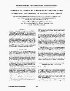
Downlink Signal Intended for User 1 Downlink Signal Intended for User 2 Uplink Signal from User 1 Uplink Signal from User 2 User 1 Base Station User 2

Figure 1: An illustration of a multiple-user MIMO channel with uplink and downlink. In the uplink, the base station receives multiple interfering signals and uses their spatial properties to separate them. In the downlink, each user often receives data intended for other users, and is not able to coordinate with them. In order to share a limited amount of frequency spectrum, all multi-user communication systems use one or more of the traditional forms of multiplexing: time-division, frequency-division, and code-division. The best multiplexing scheme for a given application is dependent on the characteristics of the particular channel of interest. The use of antenna arrays in a multi-user channel enables one further type of multiplexing often referred to as spatial multiplexing. Spatial multiplexing is particularly appealing because it can easily be used in conjunction with other forms of multiplexing to dramatically improve the number of users that can share a given channel. In addition to the promise of improved capacity for future communication networks, in some cases these methods can be applied to existing communication protocols, thus extending their usefulness. The problem of MIMO communications in multi-user environments can be further divided into two distinct problems, each with unique challenges: the “uplink” channel and “downlink” channel, as illustrated in Figure 1. The uplink refers to the case where a group of users sharing the same channel (representing a unique time slot, frequency, or code sequence) transmit simultaneously. Among information theorists this is commonly labeled the multiple access channel. This scenario requires the multi-antenna base station to successfully separate all of the interfering signals, which can be achieved if the users are transmitting from different locations by exploiting the differing spatial characteristics of the respective channels at the receiver. The downlink channel (the broadcast channel among information theorists) refers to the case where the base station transmits simultaneously to more than one user over a shared channel. This poses challenges that are somewhat different from the uplink channel, because the receivers are unable to cooperate, so the signals at the different receivers can not be processed jointly. Since 2

the receivers pictured in Figure 1 have multiple antennas, they could in theory use multiple-user detection (MUD) techniques to avoid the interfering signals. This is typically computationally costly, and in cases where users have only a single antenna, it is not possible without relying on other forms of multiplexing such as CDMA. Ideally, then, we would like to mitigate the multipleaccess interference (MAI) at the transmitter by intelligently designing the transmitted signal. In this chapter, we begin by reviewing the problem of the multi-user MIMO downlink and discuss in general terms several different transmission approaches that have been proposed. We compare the performance of some of the schemes in randomly-generated channels under ideal conditions. We then show how the algorithms would perform under real-world conditions using measurement data from an indoor propagation environment and two different outdoor environments. We focus in particular on the achievable capacity, the ability of the channels to support multiple sub-channels per user, the required separation distance between users to maximize available capacity, and the effects of channel estimation error due to user mobility. We begin with a mathematical model used for characterizing multi-user MIMO channels.

2

The Multiple-User MIMO Channel

A MIMO channel with nT transmitters and nR receivers is commonly represented as a matrix H of dimension nR × nT , where each of the coefficients [H]i,j represents the complex transfer function from the j th transmitter to the ith receiver. We denote the signal transmitted from the j th transmitter at time t as xj (t), and represent the total transmitted signal with the vector x(t) of dimension nT . Likewise, we represent the received signal with the nR -dimensional vector y(t), which can be expressed as a function of the transmitted signal, the channel matrix, and an nR -dimensional additive noise vector n(t): y(t) = Hx(t) + n(t) . (1) For simplicity, we will omit the dependence on time, referring to the transmitted and received signals instead as x and y. In a single-user point-to-point MIMO link, all outputs are available to the receiver for processing. In the multiple-user case, the nR receivers are distributed among different users, so we extend the model to reflect this. Let K represent the number of users sharing a channel, and let nR j represent the number of antennas for user j, so that the total number of P receive antennas nR = K j=1 nR j . The channel between the base and user j is now the nR j × nT matrix Hj , whose rows we denote by h∗ij as follows: £ Hj = h1j · · ·

hnR j j

¤∗

,

where (·)∗ is used to denote the complex conjugate (Hermitian) transpose. Note that this model is based on the assumption of a flat-fading or narrowband channel, which is not true in many current and next-generation wireless communications applications. This matrix channel model can still be applied to many broadband channels. For example, many modern broadband communication protocols are based on orthogonal frequency division multiplexing (OFDM). Typically, the bandwidth of one OFDM subcarrier is narrow enough that the narrowband model applies, so MIMO processing algorithms could be applied independently for each subcarrier. While

3

we assume a narrowband channel throughout this chapter, the methods discussed here can also be applied to broadband channels using OFDM or similar techniques. Using this model, consider the signal received by user j. User j not only receives its own signal through the channel Hj , but also contributions from the signals intended for other users: yj =

K X

Hj xk + nj ,

(2)

k=1

where nj is assumed to be spatially white noise. The transmitted signal x is then the sum of the PK transmitted signals for each user: x = j=1 xj . We assume that the transmitted signal xj is formed from a vector dj of mj symbols to be transmitted to user j. In a single-user channel, the number of symbols transmitted in parallel is limited by the rank of the channel matrix. Likewise, in a multi-user channel, mj is limited by the rank of Hj . We use the vector d to denote the data symbols transmitted to all users: ¤T £ d = dT1 dT2 . . . dTK , P where the dimension of d is m = K j=1 mj . It is possible to transmit at different rates to each of the K users by the choice of symbol constellation and channel coding for each users, and by the number of data streams mj transmitted to each user. Suitable values for m1 , · · · , mK will not only depend on the desired data rate for user j, but also on the available transmit power, the achievable SINR, and the number of transmit and receive antennas. Without additional coding or P multiplexing, typically mj ≤ nR j , and mk ≤ nT . The choice of mj to obtain optimal system performance is itself an important problem which has recently been studied in [1]. The transmitted signal x is formed from d using some encoding function which we denote by fe , so that x = fe (d). The receivers use a decoding function fd do estimate the data vectors: ˆ j = fd (yj ). This scheme is illustrated in Figure 2. To describe the dimensions of a particular d channel, we use the notation {nR 1 , . . . , nR K } × nT . A system with K = 4 users having one antenna each and nT =4 transmit antennas could be written as a {1,1,1,1}×4 system. Likewise, a {1,1,2,2}×4 describes a similar case where two of the users have two antennas. The challenge of the multi-user MIMO downlink is to choose encoding and decoding functions fe and fd that optimize the use of channel resources. Specific optimization goals may include maximizing total throughput, ensuring a certain quality of service (QoS) for each user, or minimizing transmit power, among others. Achieving any of these goals requires that the transmitter have some information about the channel. From an information-theoretic point of view, a MIMO channel where the transmitter has channel state information (CSI) has a different channel capacity than the same channel without CSI. Single-user MIMO systems benefit from having CSI at the transmitter mainly when nT ≥ nR or at low SNR. On the other hand, CSI in a multi-user MIMO downlink is critical to minimizing inter-user interference under all channel conditions. Obtaining CSI is itself a challenging problem [2]. It can generally be obtained in a two-way communications system by either sending the information over the reverse link, or estimating channel parameters of the reverse link and applying them to the forward link. In this chapter, we assume that CSI is available, and we will later investigate the effects of corrupted channel information on multi-user performance. 4

Channel 1 H1 n1

d

fe (d) Precoder

x

Channel K HK nK

Receiver 1

y1

fd (y1 )

ˆ1 d

Receiver K

ˆK d

yK fd (yK )

Figure 2: An illustration of downlink multi-user processing, where each user has multiple antennas, and receives parallel data symbols. Another property of radio channels to consider is how they vary over time. The assumption that CSI is available at the transmitter usually implies that the channel is quasi-static, which has been assumed in much of the research to date on multi-user MIMO channels. This is a reasonable assumption for channel environments such as wireless local area networks (LANs), where users are mobile but do not move rapidly. Cellular telephone applications are more challenging because speeds are much higher. Downlink processing methods for channels that are quickly time-varying with limited CSI is an important problem for future research. However, the results included in Section 4 suggest that the prediction horizons for MIMO systems may be much longer than in the SISO case (which has usually proven to be too short to be useful), since multiple antennas reveal more information about the physical structure of the channel [3].

2.1 Capacity Capacity is an important tool for analysis of communication channels. In single-user MIMO channels it is common to assume a constraint on total power broadcast by all transmit antennas. For a multi-user MIMO channel, the problem is more complex. Given a constraint on the total transmitted power, it is possible to allocate varying fractions of that power to different users in the network, so a single power constraint can yield many different information rates. The result is a “capacity region” like that illustrated in Figure 3 for a two-user channel. The “corners” of the region represent allocation of 100% of the power to either one of the users. For every possible power distribution in between, there is an achievable information rate, which results in the outer boundary of the region. In Figure 3, two regions are shown: one for the case where both users have similar maximum capacity, and one for the case where they are different (due, for example, to user 2’s channel being attenuated relative to user 1, sometimes referred to as the “near-far” problem). For K users, the capacity region is characterized by a K-dimensional volume. In Figure 3, two points are indicated on the boundary of each of the two regions. One point represents the maximum achievable throughput of the entire system, or the point on the curve that maximizes the sum of all users’ information rates. It is clear that this sum capacity point does not 5

Rate for User 2

Maximum Sum Capacity Capacity Region

Equal Capacity

“Near-Far” Capacity Region Rate for User 1

Figure 3: An illustration of a multi-user capacity region. The sum capacity may penalize certain users, depending on the shape of the capacity region. always represent a fair distribution of resources among the users. The second point on the two curves is located where the curves intersect with the line C2 = C1 , and represents the maximum achievable rate such that both users have equal rates. The problem in this case is that the total throughput is substantially reduced in the “near-far” case. While the sum capacity point clearly does not convey all the relevant information about a multi-user MIMO channel, it is nevertheless a useful tool for understanding the relative capabilities of a particular transmission algorithm or channel, and will be used extensively in this chapter for that purpose. The capacity of the multi-user MIMO channel is achieved by applying a concept that originates from a paper by M. Costa [4] known as “writing on dirty paper”. Costa studied communication channels with interference and proved the somewhat surprising result that if a received signal y is defined as y = s+i+w,

(3)

where s is the transmitted signal, i is interference known deterministically to the transmitter, and w is additive white Gaussian noise, the capacity of the system is the same as if there were no interference present, regardless of how strong the interference is and whether or not it is known to the receiver. Using the dirty paper analogy, the capacity of a dirty sheet of paper is the same as that of a clean sheet if the location of the dirt is known. The implications of this result for multi-user MIMO channels with CSI available at the transmitter are clear: since the channel and the transmitted signals are all known, the transmitter knows how a signal designed for one user interferes with other users, and can design the signals for the other users to compensate. This is the basis for many of the results on capacity of the MIMO broadcast channel [5–9]. While the initial capacity results characterize the achievable rate, they only prove achievability, but do not describe how this rate is achieved. More recently, some prac6

tical transmission schemes [10–12] have been proposed that use dirty paper codes to approach the capacity of the scalar interference channel. To date, no practical application of dirty-paper codes to the downlink problem has appeared, though the techniques of [13] are related to dirty-paper coding (DPC). A simplified approach to transmission in multi-user channels is to treat all interference as noise. Clearly, this is suboptimal, but it also results in much simpler implementations. The result is that the encoder fe and decoder fd are linear functions of the data to be transmitted and the received signals, respectively. The linear class of transmission schemes can generally be viewed as a type of beamforming. Linear transmission schemes exist for a wide variety of channel configurations, while so far dirty-paper schemes have only been proposed for the special case where all receivers have one antenna nR j = 1. However, the existing dirty-paper schemes can be applied to the more general case where nRj > 1 by combining them with linear processing methods. In the next section we review some of these schemes.

3

Multi-User MIMO Transmission Schemes

As noted above, the existing schemes for transmitting from an antenna array to a group of users can be put in two broad categories: linear and non-linear. They can also be categorized as algorithms for single-antenna receivers and multi-antenna receivers. In this section we review some of the linear methods that have been proposed, and briefly discuss non-linear methods.

3.1 Linear Processing, Single-Antenna Receivers We begin with linear transmission schemes for the case where each user has only one receive antenna: nR j = 1. With only one antenna, the receiver is unable to perform any spatial interference suppression of its own, so the transmitter is responsible for precoding the data in such a way that the interference seen by each user is tolerable. We consider three techniques for solving this problem: channel inversion, regularized channel inversion, and optimal beamforming. 3.1.1

Channel Inversion

Perhaps the simplest way of managing the inter-user interference in a multi-user downlink is using the (pseudo-)inverse of the channel matrix H [14–16]. For non-square channels where nT ≥ K = nR , the transmitted signal s is s = H∗ (HH∗ )−1 Γd . (4) The matrix Γ is a diagonal matrix used to scale the power transmitted to each user. The channel inversion nulls out all inter-user interference, reducing the problem to K independent scalar channels, so the amount of power allocated to one user does not affect the others. Given a constraint on the total transmitted power ρ, Γ can be chosen in different ways to achieve different goals: allocate equal power to all users, allocate equal capacity to all users, or maximize sum capacity. Sum capacity can be maximized by computing the gain of each of the independent channels and using the water-filling algorithm to distribute the available power.

7

A very simple way of allocating the power is to set Γ = γI, where γ = 1/ρ. One problem with channel inversion arises when H is ill-conditioned. In such cases, at least one of the singular values of (HH∗ )−1 is very large, γ will be large, and the SNR at the receivers will be low. It is interesting to note the similarity between channel inversion and least-squares or “zero-forcing” (ZF) receive beamforming, which applies a dual of the transformation in (4) to the receive data. Such beamformers are well-known to cause noise amplification when the channel is nearly rank deficient. On the transmit side, ZF produces signal attenuation instead. In fact, it has been shown that in the ideal case where the elements of H are independent complex Gaussian random variables, the probability density of γ has an infinite mean [17]. It is also shown in [17] and the simulation results section of this chapter that the capacity of channel inversion does not grow linearly with K. 3.1.2

Regularized Channel Inversion

When rank-deficient channels are encountered in ZF receive beamforming, one technique to reduce the effects of noise amplification is to regularize the inverse in the ZF filter. If the noise is spatially white and an appropriate regularization value is chosen, this approach is equivalent to using a minimum mean-squared error (MMSE) criterion to design the beamformer weights. Applying this principle to the transmit side suggests the following solution: 1 s = √ H∗ (HH∗ + ζI)−1 d , γ

(5)

where ζ is the regularization parameter. When ζ 6= 0, the transmitter does not perfectly cancel out all interference. The key is to define a value for ζ that optimally trades off the numerical condition of the matrix inverse against the amount of interference that is produced. It has been shown that choosing ζ = K/ρ approximately maximizes the SINR at each receiver, and leads to linear capacity growth with K [17]. Because each user sees some interference from other users, this scheme does not allow the same flexibility as exact channel inversion in adjusting the power transmitted to each user, because a change to the power weighting for one user changes the interference seen by all other users. 3.1.3

Optimal Linear Precoders

Regularized channel inversion demonstrates that perfectly canceling out all inter-user interference is not optimal, and provides a good solution in closed form at low computational cost. However, it is still not necessarily the optimal linear beamformer. Attempting to design a set of transmit beamformers without any constraints on inter-user interference is a very challenging problem because they are all interdependent. If an optimal beamformer is designed for one user, it will produce some interference for the other users. If the interference is taken into account in designing an optimal beamformer for a second user, it will emit interference that makes the first user’s beamformer suboptimal. This suggests that the optimal solution can not be computed in closed form, but requires an iterative approach. With a zero-forcing solution, a set of independent channels is created, so the power transmitted to each user can readily be adjusted to achieve a variety of different goals, such as maximizing sum capacity or insuring equal capacity for all users given a power constraint, or minimizing power 8

Table 1: Linear Precoding for Maximum Sum Capacity 1. Initialize ρj (1) = 1 for j = 1 . . . K, D = I, ∆ = I 2. Repeat until convergence (a) M = (H∗ DH + tr(D)/ρI) H∗ ∆ p (b) W = HM ρ/ tr(M∗ M) (c) nj = |[W]j,j |2 P 2 (d) dj = 1 + K i=1,i6=j |[W]i,j | (e) [D]j,j =

nj dj (dj +nj )

(f) [∆]j,j = [W]j,j /dj

given a capacity constraint for each user. In the case where inter-user interference is allowed, the solution to each of these problems will be different. Optimal transmit beamformers have been found for a variety of different optimization criteria [18–23]. We give as an example the linear precoder that optimizes sum capacity [18], which takes the form s = (H∗ DH + ζInT )−1 H∗ ∆d .

(6)

This is similar to regularized channel inversion, but we have introduced two diagonal matrices, D and ∆, which are used respectively to weight the rows of H inside the inverse, and weight the columns of the resulting beamformer. The optimal values for these matrices, and the scale constant ζ, can be computed using the iterative algorithm given in Table 1. The sum capacity as a function of the channel matrix size for the linear precoders we have discussed so far is compared with the sum capacity of the channel and capacity of an equivalent single-user channel in Figure 4. Of all the precoders, only channel inversion fails to achieve a sum capacity that increases linearly with K and nT . Regularized channel inversion offers a substantial improvement in performance, and the optimal linear precoder (labeled capacity-optimal RCI) is even better, achieving most of the sum-capacity of the channel that is achievable using DPC. As we noted earlier, there are many situations in which optimizing sum capacity is problematic because it does not guarantee a minimum level of signal to any user. There are many other optimizations that have appeared recently in the literature that may be of greater practical interest. The “power control” problem was the first of these [19, 20], which can be stated as follows: given a set of SINR requirements for each user, compute the set of beamformers b1 , . . . , bk such that the SINR requirements are met and total transmitted power is minimized. We define γj as the SINR for user j, which can be expressed as: γj = P

b∗j H∗j Hj bj , ∗ ∗ k6=j bk Hj Hj bk + 1

(7)

where we have assumed that the noise has unit variance. The power minimization problem can be 9

30 Channel Inversion Regularized Channel Inversion Capacity-Optimal RCI Sum Capacity Single User

Capacity (bits/usr)

25 20 15 10 5 0

2

3

4

5

6 K

7

8

9

10

Figure 4: Mean sum-capacity of various precoders for uncorrelated Gaussian channels with K users and nT = K transmitters at a SNR of 10 dB. stated mathematically as min

b1 ,··· ,bK

s.t.

K X

b∗k bk

k=1

b∗j H∗j Hj bj P ≥ γj , j = 1, · · · , K . ∗ ∗ k6=j bk Hj Hj bk + 1

(8)

Solutions to this problem have been proposed in [19–21]. Other optimizations for which solutions have recently been proposed include the maximization of the SINR margin for all users given a minimum SINR requirement for each user and a total power constraint [22, 23]. In addition to the sum-capacity solution, [18] also proposes a solution for maximizing the minimum capacity for each of the individual users. This whole class of solutions requires more computation than plain or regularized inversion, but since beamformers are typically computed once for an entire block of transmitted symbols, this is still a practical solution.

3.2 Linear Processing, Multi-Antenna Receivers With only a single antenna, the receivers are not able to perform spatial interference suppression of their own, so they can only receive data over a single spatial channel. With multiple antennas, these restrictions are removed, provided that the transmitter and receiver can coordinate their spatial processing, and appropriately allocate the available spatial resources. A simple approach to this would be to apply the single-antenna techniques just described, provided that nR ≤ nT , where nR is the total number of receive antennas summed over all users. This effectively treats each receive antenna as if it were a separate user, so no joint processing among the receive antennas is required, 10

but performance is limited because the problem is overly constrained, and the number of users is limited more than necessary. Both channel inversion and regularized channel inversion limit the number of users to K ≤ nT . For optimal beamforming, it is technically possible to support cases where K > nT , but realistically this can occur only when the SINR requirements are very low. So, it is reasonable to consider nT to be the practical upper bound on the number of users. If the receivers have multiple antennas, it is still possible to support up to K = nT users by using the concept of coordinated beamforming. To illustrate this, consider the block diagram of Figure 2. Assume that the decoding function fd (yj ) for user j is a linear operator wj , so that dˆj = wj∗ yj . If the beamformers were known to the transmitter in advance, then the virtual channel which represents the transfer function from the transmitter to the output of the beamformer of user j is ¯ ∗j = wj∗ Hj . h If we collect the virtual channels for each user, we can define a virtual channel for the entire system: £ ¤ ¯1 h ¯2 . . . h ¯K ∗ ¯ = h H As long as K ≤ nT , it possible to apply any of the single-antenna algorithms described earlier to ¯ The remaining problem is determining the receive beamformers wj . This the virtual channel H. information could be obtained if the transmitter were to assume a specific approach to designing the beamformers. For example, both MMSE and MRC designs for wj are functions of only the channel and the transmit beamformers, so wj could be computed from information available to the transmitter. However, this results in a situation where the solutions to the transmit and receive beamformers are dependent on each other. This suggests the following iterative approach: 1. Assume an initial set of wj values. ¯ and the transmit beamformers. 2. Compute the virtual channel H 3. Update the receive beamformers wj . 4. Repeat steps 2 and 3 until convergence. The convergence properties of this approach will depend in general on what algorithms are used on both the transmitter and receiver side to determine the beamforming weights. The concept of beamforming that is coordinated between the transmitter and receiver is the basis for several recent multi-user transmission schemes [1, 24–29]. In single-user MIMO channels with CSI available to the transmitter, capacity is achieved by spatial multiplexing, where a number of independent sub-channels are created that carry independent streams of data. In a multi-user MIMO downlink where the receivers have multiple antennas, it is also possible to transmit multiple data streams to each user. We define mj to PK be the number of sub-channels allocated to user j, and m = j=1 mj to be the total number ˜ j , where L ˜ j is the rank of of sub-channels. The restrictions on these values are that mj ≤ L ¤T £ T T T T ˜ j = H1 . . . Hj−1 Hj+1 . . . HK , and m ≤ nT . This means that allocating multiple H sub-channels to individual users limits the total number of users that can be served. The problem 11

of choosing a good value of mj has not yet been studied extensively, but the simulation results presented later in this chapter illustrate the trade-offs involved. In the case where mj > 1, define the receiver for user j as the mj × nR j matrix Wj , and the linear precoder as the nT × m matrix £ ¤ B = B1 B2 . . . BK . where Bj is the nT × mj precoder for user j. As in the single sub-channel case, the transmit precoders Bj can be derived by selecting an initial set of receivers Wj , and alternately updating Bj and Wj until convergence is reached. In this section, we discuss two general approaches to this problem. The first is a coordinated zero-forcing approach that is a generalization of channel inversion. The second is a framework for applying other methods like regularized channel inversion or optimal beamforming in a context where users have multiple antennas. 3.2.1

Coordinated Zero-Forcing

As noted previously, in cases where the receivers have multiple antennas, it is possible to use channel inversion at the transmitter if nR ≤ nT , but this over-constrains the problem, by forcing HB to be completely diagonal. In fact, all inter-user interference can be eliminated by constraining HB to be block-diagonal (i.e., Hi Bj = 0, for i 6= j). A procedure for computing the optimal B given this constraint has been proposed [24, 30–34], but it imposes restrictions on the channel configurations that can be accommodated. In order to accommodate all possible receiver sizes, those restrictions can be eliminated using the coordinated beamforming approach: estimate the receivers Wj and force Wi∗ Hi Bj to be zero. A method for computing this iteratively, referred to as the “coordinated zero-forcing” algorithm, is listed in Table 2. The result of the coordinated zero-forcing algorithm is a set of non-interfering virtual channels. One advantage of this approach is that since the channels do not interfere, the solution is independent of the power allocation to each channel, and therefore the power allocation can be performed independently from the computation of the beamformers. There are a few special cases of the coordinated zero-forcing algorithm worth noting. First, if nR j = 1 for all users, n the solution is equivalent to o channel inversion with optimal power allocation. ˜ 1 ), · · · , rank(H ˜ K ) , the convergence criterion is reached at the first Second, if nT > max rank(H step, and the solution is equivalent to the block-diagonalization solution of [24]. Third, if mj = 1 for all users, the receiver beamformers Wj are equivalent to maximal ratio combiners, and the ¯ (this allows for some computational savings solution for B is equivalent to channel inversion of H over the generalized implementation). 3.2.2

General Coordinated Beamforming

As noted in the discussion of channel inversion, the use of zero-forcing at the transmitter has some disadvantages, so there are good reasons to use other beamforming methods at the transmitter. This can be done in channels where the receivers have multiple antennas by applying the same general approach as in coordinated zero-forcing. A general algorithm for doing this is listed in Table 3.

12

Table 2: Coordinated Zero-Forcing Algorithm 1. For each user, initialize Wj as the mj dominant left singular vectors of Hj , and define ¯ j = Wj∗ Hj . H £ T ¤ ˜ ˜ (0) represent an ¯1 ... H ¯ Tj−1 H ¯ Tj+1 . . . H ¯ TK T , let V ¯j = H ¯ 2. For each user, define H j ˜ ¯ orthogonal basis for the right null space of Hj , and compute the SVD h i h iH (0) (1) (0) (1) (0) ˜ ¯ , Hj Vj = Uj Uj Σj Vj Vj (1)

(1)

where Uj and Vj represent the first mj left and right singular vectors. Update the trans(1) (1) mitter and receiver beamformers: Wj = Uj and Bj = Vj , and define 

 W1∗ H1 ¤  £ .. S=  B1 . . . BK . ∗ WK HK 3. Repeat step 2 until min P

i=1,...,K

[S]i,i Abscissa

1

0.8

{2,2}×4, mj = 2

0.6

0.4

{2,2}×4, mj = 1 {1,1}×4, mj = 1

0.2

0

Zero Forcing RCI Capacity-Optimal RCI 5

6

7

8 9 10 Capacity (bits/sec/Hz)

11

12

13

Figure 8: CCDFs of capacity for zero-forcing and regularized channel inversion in uncorrelated Gaussian channels at a SNR of 10 dB. ing using regularized channel inversion at the transmitter and MMSE receivers, and coordinated beamforming using capacity-optimal RCI at the transmitter with MMSE receivers. Note that for mj = 1, and in about 40% of cases where mj = 2, zero-forcing has slightly better performance than RCI. The reason for this is that with the ZF solution the power for each user was adjusted to maximize sum capacity, while this is not possible with RCI without using the iterative algorithm. The capacity is quite similar for all algorithms for mj = 1, but for mj = 2, it is clear that the capacity-optimal RCI method makes far better use of the second spatial sub-channel than either of the others. In some cases, as will be seen with the data-derived results, adding the second subchannel does not provide any additional benefit because of the channel characteristics. Another reason it may be preferable to use less than all available sub-channels is that this allows additional degrees of freedom in optimizing the transmission to other users. In Figure 4 (see also [17, 37]), a comparison of capacity for channel inversion and regularized channel inversion for channels where K = nT revealed that RCI, and capacity-optimal RCI achieve linear growth in capacity with K while channel inversion does not. In Figure 9, we assume that nT is fixed at 10 antennas, and compare the sum capacity of channel inversion and RCI with the theoretical limits as a function of K. In this case, the theoretical limits increase with the number of users, but the linear processing schemes achieve maximum capacity at 6 users, and channel inversion actually loses a substantial amount of capacity as K → nT . This is due to the fact that the power scaling in (4) is limited by singular values of (HH∗ )−1 , which for random complex Gaussian matrices are not well-conditioned when H is square [17]. Figure 10 compares the same three linear precoders in the context of multi-antenna receivers, with the number of data streams per user mj fixed at 1. While there is a sizable gap between zeroforcing and the RCI regularized channel inversion when the receivers have only one antenna, the difference becomes much smaller as a function of the number of receive antennas, to the point that 18

30 Channel Inversion Regularized Channel Inversion Optimal RCI Sum Capacity Single User Capacity

28

Capacity (bits/usr)

26 24 22 20 18 16 14 12 10 8

2

3

4

5

6 K

7

8

9

10

Figure 9: Comparison of capacity for channel inversion and regularized channel inversion with the sum capacity of the channel and capacity of the equivalent single-user channel for K users and nT = 10 at a SNR of 10 dB.

35 Zero Forcing Regularized Channel Inversion Capacity-Optimal RCI

Capacity (bits/sec/Hz)

30

nRj =3 25

nR j =2

20 nRj =1

15 10 5 0

2

3

4

5

6 K

7

8

9

10

Figure 10: Capacity comparison of coordinated zero-forcing and regularized channel inversion for mj = 1 and varying values of nRj for K users at a SNR of 10 dB.

19

16 14 Capacity (bits/sec/Hz)

nRj = 3 12 nRj = 2

10 8

nR j = 1

6 4

Zero Forcing Regularized Channel Inversion Capacity-Optimal RCI

2 0

0

2

4

6 8 10 12 Channel Estimation Error (dB)

14

16

Figure 11: Capacity comparison as a function of channel estimation error. it becomes almost negligible for nR j = 3. In multi-user MIMO channels, optimal transmission schemes depend heavily on the availability of CSI at the transmitter. In practice, CSI will likely be corrupted by noise. Figure 11 shows the effects of channel estimation error on performance. In this case, the error is modeled as an additive ˆ = H + N. The error is quantified by the ratio of error matrix N such that the estimated channel H the total power in H to the total power in N: kHk2F /kNk2F . It is apparent from the curves in Figure 11, that receivers with additional antennas reach their maximum capacity with more error in their channel estimates than those with only one antenna. With one antenna per user, not only do the RCI precoders significantly outperform zero-forcing, they are much more robust in the presence of channel estimation error.

5.2 Multi-User Performance in Channels Derived from Measurements While uncorrelated Gaussian channels are useful as an analysis tool, this assumption is a bestcase scenario, and it is important to also consider the specific channel conditions in which these algorithms are likely to be used. For example, if two users are located close together, their channels will likely be highly correlated, which will affect the transmitter’s ability to achieve signal separation with precoding. An important question then is what physical spacing is required to achieve the capacity levels of uncorrelated users. For indoor environments, this problem was recently studied using both channel measurements and statistical models [38, 39]. In this section, we compare performance derived from the indoor measurements with outdoor measurements and random Gaussian channels. The transmission scheme in all cases is coordinated beamforming with MMSE receivers and capacity-optimal RCI at the transmitter, so the capacity referred to here is the maximum achievable throughput given linear precoding and decoding. We consider three important questions. First, we test how closely two users can be located in space before a significant 20

11

Capacity (bits/sec/Hz)

10

9

8

7

6

nR j = 1, mj = 1 nRj = 2, mj = 1 nR j = 2, mj = 2 0

2

4 6 Separation (wavelengths)

8

10

Figure 12: Mean system capacity as a function of separation distance for a two-user MIMO channel derived from indoor measurement data. Markers on the right side are capacity for random separation, and along the left side are for uncorrelated Gaussian channels. reduction in spatial multiplexing performance is observed. Second, we test channels with many users to see how much multipath is present in the channel and how many users can be supported, and third, we test how far a receiver terminal can move before updated CSI is required. 5.2.1

Effects of Inter-User Separation

We begin by examining the performance of two-user channels. Figure 12 shows the capacity as a function of separation distance for coordinated beamforming using regularized channel inversion for indoor channels. The cases shown are for nRj = 1, and nRj = 2 with mj = 1 and 2. As a reference, the mean capacity was computed for uncorrelated Gaussian channels and for measured channels where the users’ locations were chosen randomly from anywhere in the data set were computed, and those values are shown along the left and right sides of the plot, respectively. While random spacing allows slightly higher capacity than fixed spacing, capacity for fixed spacing in all three cases appears to reach its maximum at a separation of 5 wavelengths. For the 2.43 GHz channel we are considering, this is equivalent to about 60 cm. For both cases where mj = 1, the capacity from measured data is very close to that of uncorrelated Gaussian channels, but there is a gap for mj = 2. This is an indication that there is likely a greater spread in the singular values of the channel matrices for the measured data than for simulated random channels. Causes of this include correlation between antenna elements and a dominant path in the multipath environment. Figure 13 shows the mean capacity as a function of user separation for the two outdoor channels. Outdoor channel A, which is almost entirely NLOS with multiple buildings in the vicinity, achieves higher overall capacity and the maximum capacity appears to be reached at 5 wavelengths, as in the indoor case. Channel B, on the other hand, which consists of LOS channels, requires about 21

10

Capacity (bits/sec/Hz)

9 8 7 6 nR j = 1, mj = 1 nRj = 2, mj = 1 nR j = 2, mj = 2 Outdoor A Outdoor B

5 4 3

0

5

10 Separation (wavelengths)

15

20

Figure 13: Mean system capacity as a function of separation distance for a two-user MIMO channel derived from outdoor measurement data. 10 wavelengths to reach maximum capacity and has lower overall capacity. Even a distance of 10 wavelengths is relatively small, considering it is equivalent to about 1.2 meters at our measurement frequency. Since the channels have all been normalized, relative attenuation between the different propagation environments is not considered here. It is also interesting to note that when nRj = 2, outdoor channel A achieves a small increase in capacity when mj = is increased from 1 to 2 (but a smaller increase than the indoor environment), but channel B does not. This is an indicator that channel B has virtually no multipath diversity–the channel is almost always dominated by a single multipath component–and Channel A has less multipath diversity than the indoor channel. In Figure 14, we consider the performance of a system with a larger number of transmit antennas as a function of the number of users sharing the channel. We compare the performance of uncorrelated Gaussian channels with locations randomly selected from the data sets as a function of the number of users for nR j = 1 and 3, with mj = 1. The random Gaussian channel outperforms the measured channels by a larger margin for multi-antenna receivers than for single-antenna receivers. For multi-antenna receivers, the indoor channel achieves performance close to that of random channels except for 6 and 7 users. For both outdoor channels, there is significantly less capacity than random channels for as few as 4 users. This illustrates that regardless of the number of transmitters and users, the system capacity in real propagation environments may be limited by the multipath structure. Beyond a certain limit (defined by the multipath diversity of the channel) the addition of transmit and receive antennas results mainly in beamforming gain rather than diversity or multiplexing gain.

22

26 IID Channel Indoor Channel Outdoor Channel A Outdoor Channel B nR j = 1 nRj = 3

Capacity (bits/sec/Hz)

24 22 20 18 16 14 12 10

3

4

5 Number of Users

6

7

Figure 14: Sum capacity of coordinated beamforming with optimal RCI for multi-user channels with 7 transmit antennas and users placed at random locations. 5.2.2

Effects of User Motion

In Figure 11, we demonstrated that noise in the CSI does not measurably degrade performance if the energy in H is greater than the noise in the channel estimate by about 12 dB. In this section, we assume that the noise effects are negligible and measure the effects of errors in the CSI due to user motion. We assume that CSI is made available to the transmitter via a feedback channel, but the receiver may have moved by the time the transmitter has processed the channel estimate. A similar case was considered in [40]. In [39], this scenario was studied for a {2,2}×4 channel with mj = 2 in an indoor environment. Because we observe better overall performance with mj = 1, we consider here the case of {1,1}×4 channels and {2,2}×4 channels with errors in CSI. The sum capacity at 10 dB SNR as a function of separation distance from CSI measurement to CSI usage is shown for the indoor and both outdoor channels in Figure 15. In the first 0.25 wavelengths, the degradation is steeper for outdoor channels than for indoor channels, while the rate is similar for all of the channels from 0.25 to 1 wavelength. The slope of the curves for larger separations appears to be less steep for nR j = 2. This can be attributed to the fact that the dominant eigenvector of each user’s channel is closely related to the angle of strongest propagation path, which will tend to change more slowly than the individual channel coefficients. This is another advantage of adding additional antennas at the receivers. In general the effects of CSI error appear to be similar for both the indoor and outdoor environments studied here. It is possible to compensate for these errors up to a certain point by adding additional SINR margin to the design requirements for transmit beamformers. This type of CSI error is a limited problem in indoor environments because mobility speeds are quite low. The slightly higher sensitivity to CSI error in outdoor environments combined with higher speeds imply that CSI will not be useful for long periods of time, making the problem of obtaining relevant CSI at

23

9 Indoor Outdoor A Outdoor B

Capacity (bits/sec/Hz)

8 7

nRj = 2

6 5 4

nRj = 1

3 2

0

0.2

0.4 0.6 Separation (wavelengths)

0.8

1

Figure 15: Mean capacity as a function of distance between a user’s actual location and the location of the available channel estimate. the transmitter a more significant challenge for outdoor channels than indoor.

6

Summary

Spatial multiplexing algorithms in multi-user MIMO systems can substantially increase the capacity of a wireless network, assuming that accurate CSI is available, and that the channels for different users are uncorrelated. In this chapter, we have reviewed some of the available algorithms for the downlink, and demonstrated the expected performance in both ideal uncorrelated Gaussian channels and channels derived from measurements of both indoor and outdoor propagation environments. While many of the multiplexing algorithms proposed so far are designed for the case where each user has only one antenna, they can be readily adapted to cases where the users have more than one antenna by using linear processing at the receiver to reduce the dimension of the channel. The results demonstrate a clear benefit from adding a second or third antenna to each user and using simple processing schemes at the receiver such as MMSE beamforming. When users have more than one antenna and coordinated beamforming is used, the performance gaps between transmission approaches such as channel inversion and regularized channel inversion become much smaller. In practice, achieving spatial multiplexing requires that users’ channels be sufficiently uncorrelated, which implies a certain minimum separation between them. For indoor propagation measurements tested here, a spacing of about 5 wavelengths (approximately 60 cm at the measurement frequency) appears to be sufficient, regardless of the number of users, while in outdoor environments with significant multipath, a spacing of 5-10 wavelengths (0.6-1.2 m) is sufficient depending on the environment. 24

While in uncorrelated Gaussian channels, system capacity can grow linearly with the number of transmit antennas and number of users, the multipath structure encountered in measured channels imposes limits on how many users can be multiplexed spatially. In the particular indoor environment measured here, with a base station array of 7 elements, most of the available capacity is reached at around 5-6 users, while the number is 3-4 for the outdoor environments that were studied here. This limit is a function of the number of significant multipath components for each user and the difference in multipath structures for users located near each other. All of the measurement results were taken over limited paths, so it is possible that more users can be supported if they are scattered over a wider area. The use of CSI at the transmitter in multi-user MIMO downlinks appears to be particularly challenging in outdoor propagation environments because performance quickly becomes degraded when the channel has changed relative to the available CSI. Protocols that use spatial multiplexing in outdoor MIMO downlinks will therefore use CSI for very short time horizons.

Acknowledgments This work was supported by the U.S. Army Research office under the Multi-University Research Initiative (MURI) grant W911NF-04-1-0224, by the DARPA Advanced Technology Office, and by San Diego Research Center, Inc.

References [1] R. L.-U. Choi, M. T. Ivrlaˇc, R. D. Murch, and J. A. Nossek, “Joint transmit and receive multi-user MIMO decomposition approach for the downlink of multi-user MIMO systems,” in Proceedings of the IEEE 58th Vehicular Technology Conference. Orlando, FL: IEEE, October 6-9 2003. [2] D. J. Love, R. W. Heath Jr., W. Santipach, and M. L. Honig, “What is the value of limited feedback for MIMO channels?” IEEE Communications Magazine, vol. 42, no. 10, pp. 54–59, October 2004. [3] T. Svantesson and A. L. Swindlehurst, “A performance bound for prediction of a multipath MIMO channel,” in Proc. 37th Asilomar Conference on Signals, Systems, and Computers, Session: Array Processing for Wireless Communications, Pacific Grove, CA, November 2003. [4] M. Costa, “Writing on dirty paper,” IEEE Trans. Information Theory, vol. 29, pp. 439–441, May 1983. [5] G. Caire and S. Shamai, “On the achievable throughput of a multi-antenna Gaussian broadcast channel,” IEEE Transactions on Information Theory, vol. 43, pp. 1691–1706, July 2003. [6] W. Yu and J. Cioffi, “Sum capacity of a Gaussian vector broadcast channel,” in Proceedings IEEE International Symposium on Information Theory, July 2002, p. 498. 25

[7] P. Viswanath and D. Tse, “Sum capacity of the vector Gaussian broadcast channel and uplinkdownlink duality,” IEEE Transactions on Information Theory, vol. 49, no. 8, pp. 1912–1921, August 2003. [8] S. Vishwanath, N. Jindal, and A. Goldsmith, “Duality, achievable rates and sum capacity of Gaussian MIMO broadcast channels,” IEEE Transactions on Information Theory, vol. 49, no. 10, pp. 2658–2668, August 2003. [9] H. Weingarten, Y. Steinberg, and S. Shamai, “The capacity region of the Gaussian MIMO broadcast channel,” in Proceedings Conf. on Information Sciences and Systems (CISS), Princeton, NJ, March 2004. [10] G. Caire and S. Shamai, “LDPC coding for interference mitigation at the transmitter,” in Proc. 40th annual Allerton Conference on Communication, Control, and Computing, October 2002. [11] ——, “Writing on dirty tape with LDPC codes,” in Multiantenna Channels: Capacity, Coding and Signal Processing, ser. DIMACS Series in Discrete Mathematics and Theoretical Computer Science, vol. 62, 2002, pp. 123–140. [12] T. Philosof, U. Erez, and R. Zamir, “Precoding for interference cancellation at low SNR,” in 22nd Convention of IEEE Israel Section, Tel-Aviv University, December 2002. [13] B. M. Hochwald, C. B. Peel, and A. L. Swindlehurst, “A vector-perturbation technique for near-capacity multi-antenna multi-user communication—part II: Perturbation,” IEEE Transactions on Communications, vol. 53, no. 3, pp. 537–544, March 2005. [14] J. H. Winters, J. Salz, and R. D. Gitlin, “The Impact of Antenna Diversity on the Capacity of Wireless Communication Systems,” IEEE Transactions on Communications, vol. 42, no. 2, pp. 1740–1751, Feb/Mar/Apr 1994. [15] D. Gerlach and A. Paulraj, “Adaptive transmitting antenna arrays with feedback,” IEEE Signal Processing Letters, vol. 1, no. 10, pp. 150–152, October 1994. [16] T. Haustein, C. von Helmolt, E. Jorwieck, V. Jungnickel, and V. Pohl, “Performance of MIMO systems with channel inversion,” in Proceedings of the IEEE 55th Vehicular Technology Conference, vol. 1, Birmingham, AL, May 2002, pp. 35–39. [17] C. B. Peel, B. M. Hochwald, and A. L. Swindlehurst, “A vector-perturbation technique for near-capacity multiantenna multiuser communication-part I: Channel inversion and regularization,” IEEE Transactions on Communications, vol. 53, no. 1, pp. 195–202, January 2005. [18] M. Stojnic, H. Vikalo, and B. Hassibi, “Rate maximization in multi-antenna broadcast channels with linear preprocessing,” in Proceedings of IEEE Globecom, November 2004, pp. 3957–3961. [19] F. Rashid-Farrokhi, K. R. Liu, and L. Tassiulas, “Transmit beamforming and power control for cellular wireless systems,” IEEE Journal on Selected Areas in Communications, vol. 16, no. 8, pp. 1437–1450, October 1998. 26

[20] E. Visotsky and U. Madhow, “Optimum beamforming using transmit antenna arrays,” in Proceedings of the IEEE Vehicular Technology Conference, vol. 1. Houston, TX: IEEE, May 16-20 1999, pp. 851–856. [21] M. Bengtsson and B. Ottersten, “Optimal and suboptimal beamforming,” in Handbook of Antennas in Wireless Communications, L. Godara, Ed. CRC Press, August 2001. [22] H. Boche and M. Schubert, “Multi-antenna downlink transmission with individual SINR receiver constraints for cellular wireless systems,” in Proceedings of the 4th International ITG Conference on Source and Channel Coding, Informationstechnische Gesellschaft im VDE (ITG). VDE Verlag GmbH, January 2002, pp. 159–166. [23] M. Schubert and H. Boche, “Solution of the multiuser downlink beamforming problem with individual SINR constraints,” IEEE Transactions on Vehicular Technology, vol. 53, no. 1, pp. 18–28, January 2004. [24] Q. H. Spencer, A. L. Swindlehurst, and M. Haardt, “Zero-forcing methods for downlink spatial multiplexing in multi-user MIMO channels,” IEEE Transactions on Signal Processing, vol. 52, no. 2, February 2004. [25] J.-H. Chang, L. Tassiulas, and F. Rashid-Farrokhi, “Joint transmitter receiver diversity for efficient space division multiaccess,” IEEE Transactions on Wireless Communications, vol. 1, no. 1, pp. 16–27, January 2002. [26] Z. Pan, K.-K. Wong, and T. Ng, “MIMO antenna system for multi-user multi-stream orthogonal space division multiplexing,” in Proceedings of the IEEE International Conference on Communications, vol. 5. Anchorage, Alaska: IEEE, May 2003, pp. 3220–3224. [27] K.-K. Wong, R. Murch, and K. B. Letaief, “A joint-channel diagonalization for multiuser MIMO antenna systems,” IEEE Trans. Wireless Comm., vol. 2, no. 4, pp. 773–786, July 2003. [28] Q. H. Spencer, A. L. Swindlehurst, and M. Haardt, “Fast power minimization with QoS constraints in multi-user MIMO downlinks,” in Proceedings of the IEEE International Conference on Acoustics, Speech, and Signal Processing. IEEE, April 2003. [29] Q. H. Spencer and A. L. Swindlehurst, “A hybrid approach to spatial multiplexing in multi-user MIMO downlinks,” EURASIP Journal on Wireless Communications and Networking, vol. 2004, no. 2, pp. 236–247, December 15 2004. [Online]. Available: http://wcn.hindawi.com/volume-2004/issue-2.html [30] R. L.-U. Choi and R. D. Murch, “A downlink decomposition transmit pre-processing technique for multi-user MIMO systems,” in Proceedings of IST Mobile & Wireless Telecommunications Summit, June 2002. [31] A. Bourdoux and N. Khaled, “Joint Tx-Rx optimization for MIMO-SDMA based on a nullspace constraint,” in Proc. IEEE Vehic. Tech. Conf., September 2002, pp. 171–174. 27

[32] Q. H. Spencer and M. Haardt, “Capacity and downlink transmission algorithms for a multiuser MIMO channel,” in Conference Record of the 36th Asilomar Conference on Signals, Systems and Computers. IEEE, November 2002. [33] M. Rim, “Multi-user downlink beamforming with multiple transmit and receive antennas,” Electronics Letters, vol. 38, no. 25, pp. 1725–1726, 5th December 2002. [34] R. Choi and R. Murch, “A transmit preprocessing technique for multiuser MIMO systems using a decomposition approach,” IEEE Trans. Wireless Comm., vol. 3, no. 1, pp. 20–24, January 2004. [35] V. Stankovic, M. Haardt, and M. Fuchs, “Combination of block diagonalization and THP transmit filtering for downlink beamforming in multi-user MIMO systems,” in Proc. European Conference on Wireless Technology (ECWT 2004), Amsterdam, The Netherlands, Oct. 2004, to be published. [36] J. W. Wallace, M. A. Jensen, A. L. Swindlehurst, and B. D. Jeffs, “Experimental characterization of the MIMO wireless channel: Data acquisition and analysis,” IEEE Transactions on Wireless Communications, vol. 2, no. 2, pp. 335–343, March 2003. [37] Q. H. Spencer, C. B. Peel, A. L. Swindlehurst, and M. Haardt, “An introduction to the multiuser MIMO downlink,” IEEE Communications Magazine, vol. 42, no. 10, pp. 60–67, October 2004. [38] Q. Spencer and T. Svantesson, “MIMO downlink spatial multiplexing algorithms applied to channel measurements,” in Proceedings of the IEEE 58th Vehicular Technology Conference. Orlando, FL: IEEE, October 6-9 2003. [39] Q. H. Spencer, T. Svantesson, and A. L. Swindlehurst, “Performance of MIMO spatial multiplexing algorithms using indoor channel measurements and models,” Wireless Communications and Mobile Computing, vol. 4, no. 7, pp. 739–754, November 2004. [40] P. Zetterberg, M. Bengtsson, D. McNamara, P. Karlsson, and M. A. Beach, “Performance of multiple-receive multiple-transmit beamforming in WLAN-type systems under power or EIRP constraints with delayed channel estimates,” in Proceedings of the 55th Vehicular Technology Conference, vol. 4. IEEE, 2002, pp. 1906–1910.

28