Phase Transitions of Soft Disks in External Periodic Potentials: A ...

arXiv:cond-mat/0209363v1 [cond-mat.stat-mech] 16 Sep 2002

Phase Transitions of Soft Disks in External Periodic Potentials: A Monte Carlo Study W. Strepp1 , S. Sengupta2 , P. Nielaba1 1 2

Physics Department, University of Konstanz, Fach M 691, 78457 Konstanz, Germany

S.N. Bose National Centre for Basic Sciences, Block JD, Sector III, Salt Lake, Calcutta 700098, India

Abstract The nature of freezing and melting transitions for a system of model colloids interacting by a DLVO potential in a spatially periodic external potential is studied using extensive Monte Carlo simulations. Detailed finite size scaling analyses of various thermodynamic quantities like the order parameter, its cumulants etc. are used to map the phase diagram of the system for various values of the reduced screening length κas and the amplitude of the external potential. We find clear indication of a reentrant liquid phase over a significant region of the parameter space. Our simulations therefore show that the system of soft disks behaves in a fashion similar to charge stabilized colloids which are known to undergo an initial freezing, followed by a re-melting transition as the amplitude of the imposed, modulating field produced by crossed laser beams is steadily increased. Detailed analysis of our data shows several features consistent with a recent dislocation unbinding theory of laser induced melting.

1

I. INTRODUCTION

The liquid-solid transition in two dimensional systems of particles under the influence of external modulating potentials has recently attracted a fair amount of attention from experiments [1–7], theory [8,9] and computer simulations [10–13]. This is partly due to the fact that well controlled, clean experiments can be performed using colloidal particles [16] confined between glass plates (producing essentially a two-dimensional system) and subjected to a spatially periodic electromagnetic field generated by interfering two, or more, crossed laser beams. One of the more surprising results of these studies, where a commensurate, one dimensional, modulating potential is imposed, is the fact that there exist regions in the phase diagram over which one observes reentrant [4–6] freezing/melting behavior. As a function of the laser field intensity the system first freezes from a modulated liquid to a two dimensional triangular solid. A further increase of the intensity confines the particles strongly within the troughs of the external potential, suppressing fluctuations perpendicular to the troughs, which leads to an uncoupling of neighboring troughs and to re-melting. Our present understanding of this curious phenomenon has come from early mean field density functional [8] and more recent dislocation unbinding [9] calculations. The mean field theories neglect fluctuations and therefore cannot explain reentrant behavior. The order of the transition is predicted to be first order for small laser field intensities, though for certain combinations of external potentials (which includes the specific geometry studied in the experiments and in this paper) the transition may become second order after going through a tricritical point. In general, though mean field theories are applicable in any dimension, the results are expected to be accurate only for higher dimensions and long ranged potentials. The validity of the predictions of such theories for the system under consideration is, therefore, in doubt. A more recent theory [9] extends the dislocation unbinding mechanism for twodimensional melting [24,25] to systems under external potentials. For a two-dimensional triangular solid subjected to an external one-dimensional modulating potential, the only 2

dislocations involved are those which have their Burger’s vectors parallel to the troughs of the potential. The system, therefore, maps onto an anisotropic, scalar Coulomb gas (or XY model) [9] in contrast to a vector Coulomb gas [24,25] for the pure 2D melting problem. Once bound dislocation pairs are integrated out, the melting temperature is obtained as a function of the renormalized or “effective” elastic constants which depend on external parameters like the strength of the potential, temperature and/or density. Though explicit calculations are possible only near the two extreme limits of zero and infinite field intensities, one can argue effectively that a reentrant melting transition is expected on general grounds quite independent of the detailed nature of the interaction potential for any two-dimensional system subject to such external potentials. The actual extent of this region could, of course, vary from system to system. In addition, these authors predict that the autocorrelation function of the Fourier components of the density (the Debye-Waller correlation function) decays algebraically in the solid phase at the transition with an universal exponent which depends only on the geometry and the magnitude of the reciprocal lattice vector. Computer simulation results in this field have so far been inconclusive. Early simulations [10] involving colloidal particles interacting via the Derjaguin, Landau, Verwey and Overbeek (DLVO) potential [16] found a large reentrant region in apparent agreement with later experiments. On closer scrutiny, though, quantitative agreement between simulation and experiments on the same system (but with slightly different parameters) appears to be poor [6]. Subsequent simulations [11–13] have questioned the findings of the earlier computation and the calculated phase diagram does not show a significant reentrant liquid phase. Motivated, in part, by this controversy, in Ref. [14] we have recently investigated the freezing/melting behavior of a two dimensional hard disk system in an external potential. The pure hard disk system is rather well studied [17–20] by now and the nature of the melting transition in the absence of external potentials reasonably well explored. Also, there exist colloidal systems with hard interactions [16] so that, at least in principle, actual experiments using this system are possible. Finally, a hard disk simulation is relatively cheap to implement and one can make detailed studies of large systems without straining 3

computational resources. By these calculations we obtained a clear signature of a reentrant liquid phase showing that this phenomenon is indeed a general one as indicated in Ref. [9]. In the present paper we studied a system of particles interacting by a DLVO potential in a external periodic potential, motivated on one hand whether this reentrance scenario is dependent on the range of interaction, and on the other hand to compare it with experimental results [6]. The phase diagram has been computed by an application of finite size scaling methods similar to the methods used in our study of the hard disk systems in external potentials [14]. The rest of our paper is organized as follows. In Section II we specify the model and the simulation method including details of the finite size analysis used. In Section III we present our results for both zero and non-zero external potential, in particular results for the order parameter and its cumulants with a discussion on finite size effects. We also present other quantities like order parameter susceptibility, correlation functions and heat capacity, which further illustrates the nature of the phase transitions in this system. In Section IV we discuss our work in relation to the existing literature on this subject, summarize and conclude.

II. MODEL AND METHOD

A. The Model

1. Potentials

We study a system of N soft disks in a two dimensional box of fixed volume interacting with the DLVO pair potential φ(rij ) [16] between particles i and j with distance rij , 2 exp(κR) exp(−κrij ) , (1) 1 + κR rij q P 2 where R is the radius of the particles, κ = ǫ0 ǫrekB T i ni zi2 is the inverse debye screening (Z ∗ e)2 φ(rij ) = 4πǫ0 ǫr



length, Z ∗ is the effective surface charge, and ǫr is the dielectric constant of water. We used 4

ǫr = 78 and, unless otherwise indicated, 2R = 1.07µm and Z ∗ = 7800. Additionally we chose a temperature of T = 293.15K, and the particle density such that the particle spacing of an ideal lattice is as = 2.52578µm. We then obtain different values for the reduced inverse screening length κas by varying κ as needed. In our simulation we set 2R to be the unit length. The potential in eq. (1) mainly depends on the value of κas , so all features found for this system should be valid also for slightly different values of the other parameters mentioned above. In addition a particle with coordinates (x, y) is exposed to an external periodic potential of the form: V (x, y) = V0 sin (2π x/d0 )

(2)

The constant d0 in Eq.(2) is chosen such that, for a density ρ = N/Sx Sy , the modulation is commensurate to a triangular lattice of disks with nearest neighbor distance as : d0 = √ as 3/2. The main parameters which define our system are κas and the reduced potential strength V0 /kB T = V0∗ , where kB is the Boltzmann constant.

2. box geometry

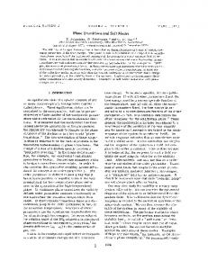
All of the data (unless otherwise indicated) presented for V0∗ < 0.2 are obtained by a √ simulation in a rectangular box of size Sx ∗ Sy (Sx /Sy = 3/2) and periodic boundary conditions in x- and y-direction, i.e. exactly as in [14]. We will refer to it as ’fixed box geometry’ in the rest of the paper. For V0∗ 6= 0 the external potential modulates the structure of the fluid and the particles form troughs oriented in the y-direction. In order to avoid unphysical results, for V0∗ ≥ 0.2 we mainly used a box with periodic boundary conditions in x-direction and movable walls in y-direction, see Fig. 1, and we will call this ’variable box geometry’. The simulation box volume is fixed as well as the side length Sx , but in x-direction the box is divided into slabs of width d0 , centered around the minima of the external periodic potential. The wall at the 5

end of each slab can move at most as upwards or downwards around its equilibrium position: |b| < as , such that each slab has variable length between Sy −2as and Sy + 2as in y-direction. √ The averaged box geometry still is Sx /Sy = 3/2 as for the fixed one. The constraint for neighboring walls is to have a distance less than as /2: |c| < as /2. The walls are hard, so no particle can cross them. This is indicated as thick solid line in Fig. 1. To accommodate the particles in the box as well as possible, additional ’boundary’ particles were placed in center (f = d0 /2) behind each wall at a distance of e = as /2. The boundary particles interact with the particles in the box by the usual DLVO potential, but do not interact with each other. The motion of the walls is done with a Monte-Carlo procedure and keeps the volume constant, so we are still in the NVT (but variable shape) ensemble. The movable walls are chosen to give the system additional degrees of freedom to relax internal stress. We were lead to this geometry by some unphysical results when using the fixed box geometry and higher particle numbers (N ≥ 4096). For a detailed discussion see end of section III B.

B. The Method

1. Numerical Details

We perform NVT Monte Carlo (MC) simulations [21,22] for the system with interactions given by Eqs. (1) and (2) for various values of V0∗ and κas . Averages < · > of observables have been obtained with the canonical measure. In order to obtain thermodynamic quantities for a range of system sizes, we analyzed various quantities within subsystems and used < · >L to denote averages in it. The subsystems are of size √ Lx × Ly where Lx and Ly are chosen as Ly = Las and Lx = Ly 3/2 = Ld0 consistent with the geometry of the triangular lattice. A subbox of size L = 3 as shown in Fig. 2 contains in average NL = L2 = 9 particles. Most of the simulations described below have been done for a total system size of N =

6

1024 and N = 4096 particles, additional ones with N = 400. Phase transitions have been studied in most cases by starting in the ordered solid and increasing κas for fixed V0∗ . Runs where κas is decreased were also performed for comparison. A typical simulation run with 107 Monte Carlo steps (MCS) per particle (including 3 ×106 MCS for relaxation) took about 50 CPU hours on a PII/500 MHz PC. In addition to ordinary (local) MC moves we also used ‘trough moves’, by which particle placements in neighboring troughs are tried. Besides producing faster equilibration, including such moves ensures that at high V0∗ the formation of dislocations is not artificially hindered since particles can in effect bypass each other more easily — this is very unlikely with purely local MC moves.

2. Observables

The potential energy of the system per particle ε is computed by: " # N X X 1 ε∗ = φ(rij ) + V (xi , yi ) NkB T i=1 j>i

(3)

and the heat capacity per particle from the fluctuations of ε∗ : cV = N < (ε∗ − < ε∗ >)2 > kB

(4)

The nature of the fluid-solid phase transition in two dimensions has been a topic of controversy throughout the last forty years [18–20,23–27]. It is well known that true long range positional order is absent in the infinitely large system due to low energy long wavelength excitations so that translational correlations decay algebraically. According to the dislocation unbinding mechanism [24–26] the two dimensional solid (with quasi long ranged positional and long ranged orientational order) first melts into a “hexatic” phase with no positional order but with quasi long ranged orientational order signified by an algebraic decay of bondorientational correlation. A second KT transition, driven by disclination unbinding, leads to melting of the hexatic into the liquid, where both the orientational and positional order 7

is short ranged. Therefore a useful order parameter in zero external field is the orientational order parameter. For a particle j located at ~rj we define the local orientational order: ψ6,j =

Nb 1 X ei6θlj Nb l=1

where Nb is the number of nearest neighbors, and θlj the angle between the axis ~rl − ~rj and an arbitrary reference axis. For the total system we use: N 1 X ψ6 = ψ6,j N j=1

and as orientational correlation function:

∗ g6 (rij ) = | < ψ6,i ψ6,j > |

In an external periodic field given by Eq.(2), however, the bond orientational order parameter is nonzero even in the fluid phase [9,12]. This is because for V0∗ 6= 0 we have now a “modulated” liquid, in which local hexagons consisting of the six nearest neighbors of a particle are automatically oriented by the external field. Thus < ψ6 > is nonzero both in the (modulated) liquid and the crystalline phase and it cannot be used to study phase transitions in this system. The order parameters corresponding to a solid phase are the Fourier components of the (non-uniform) density ρ(~r) calculated at the reciprocal lattice ~ ~ = points {G}. This (infinite) set of numbers are all zero (for G 6 0 ) in an uniform liquid phase and nonzero in a solid. We restrict ourselves to the star consisting of the six smallest reciprocal lattice vectors of the two-dimensional triangular lattice. In the modulated liquid phase that is relevant to our system, the Fourier components corresponding to two out of these six vectors, viz. those in the direction perpendicular to the troughs of the external potential, are nonzero [8]. The other four components of this set consisting of the one in ~ 1 (as defined for the ideal crystal in Fig. 2), and those equivalent to it by the direction G symmetry, are zero in the (modulated) liquid and nonzero in the solid (if there is true long range order). We therefore use the following order parameter: N 1 X ~ 1 · ~rj ) exp(iG ψG1 = N j=1 8

where ~rj is the position vector of the j th particle. The corresponding susceptibility χG1 is: kB T χG1 = L2



  (ψG1 )2 − hψG1 i2

(5)

To measure the positional correlation, we chose the Debye-Waller correlation function which we define as follows: ~ u(0)) ~ = | < eiG~ 1 (~u(R)−~ CG~ 1 (R) >|

~ points to the elementary cell of the ideal lattice, and ~u(R) ~ is the deviation of the where R ~ + ~u(R). ~ In this case we have chosen the actual particle position from the ideal lattice: ~r = R ~ to lie along the y axis (i.e. along the troughs of the potential). In the solid direction of R we expect this quantity do decay algebraically, i.e. CG~ (y) ∝ 1/y ηG~ [9,24], where ηG~ depends on the elastic constants. ψG1 is sensitive to the phase transition where positional order is lost. Therefore, when decreasing V0∗ we expect the phase boundary to converge to the corresponding transition at zero external potential. But in contrast to V0∗ 6= 0 where the crystal is oriented by the external potential, at V0∗ = 0 it is only weakly fixed by the boundary conditions and can start to rotate, so we can not apply ψG1 there. For this purpose we use a slightly modified positional order parameter ψ˜G1 at V0∗ = 0: the phase information of ψ6 (of course, before taking the absolute value) is used to determine the orientation of the crystal, and then a tilted coordinate system is used to compute ψ˜G1 . We applied the same method when calculating CG~ 1 (y) at V0∗ = 0. We have determined phase transition points by the order parameter cumulant intersection method. The fourth order cumulant UL of the order parameter distribution is given by [28]: UL (V0∗ , κas ) = 1 −

< ψx4 >L 3 < ψx2 >2L

(6)

In order to distuingish between the cumulants of ψ6 and ψG1 , we denote them with UL,6 and UL,G , respectively. In the liquid (short ranged order) UL → 1/3 and in the solid (long range order) UL → 2/3 for L → ∞. In case of a continuous transition close to the transition point the cumulant is only a function of the ratio of the system size ≈ Las and the correlation 9

length ξ: UL (Las /ξ). Since ξ diverges at the critical point the cumulants for different system sizes intersect in one point: UL1 (0) = UL2 (0) = U ∗ . U ∗ is a non-trivial value, i.e. U ∗ 6= 1/3 and U ∗ 6= 2/3. Even for first order transitions these cumulants intersect [29] though the value U ∗ of UL at the intersection is not universal any more. The intersection point can, therefore, be taken as the phase boundary regardless of the order of the transition. This is useful since the order of the melting transition in 2D either in the absence [18–20,23–27] or with [8–13] external potentials is not unequivocally settled. And there is also another aspect in our special case: since the positional order correlation is predicted to decay algebraically in the solid phase (quasi long ranged order), the whole solid can be seen as consisting of a line or area of critical points with temperature- dependent critical indices ηG~ (T ) [24]. In that case we expect the cumulants to merge at a nontrivial value at the onset of the solid phase instead of intersecting, yielding a line of intersections. We indeed observed this behavior for hard disks in high external potentials [14]. For the same reasons the same behavior is expected for the ψ6 -cumulants at the liquid-hexatic transition and in the hexatic phase [18]. Also the very similar 2d-XY-spin model shows this behavior when using the magnetization as order parameter [30]. Note that though the order parameter < ψG1 > decays to zero with increasing system size even in the 2-d solid (assuming quasi long ranged order there), the cumulants will stay at the non-trivial value regardless of L. So for L → ∞ there should be a jump from 1/3 to this nontrivial value when crossing the phase boundary from liquid to solid, which underlines the usefulness of cumulants. In order to map the phase diagram we systematically vary the system parameters V0∗ and κas to detect order parameter cumulant intersection- or merging points which are then identified with the phase boundary.

10

III. RESULTS AND DISCUSSION

A. Zero external potential

In this section we analyse the system properties for zero external field. In particular we present results for the order parameter, the cumulants, the correlation functions and the heat capacity for different values of κas . In these studies we used the fixed box geometry. In Fig. 3 the cumulant of the ψ6 order parameter versus κas is shown for different subsystem sizes. We identify the phase transition value of κ6 as at about 14.42 by locating the cumulant intersection point. Since the positional order is not well defined in two-dimensional systems, the positional order parameter ψ˜G1 shows a strong system-size dependency, see Fig. 4. The cumulants of ψ˜G1 intersect at a value of κG as ≈ 14.25, which is slightly smaller than κ6 as . This is in agreement with a KTHNY two stage melting scenario, in which the solid and the fluid phase are separated by a “hexatic” region in the phase diagram, in which the positional order is short ranged and the bond-orientational order is long ranged. Both effects are detected by the two order parameters, ψ6 being sensitive for the bond-orientational order and ψ˜G1 on the positional order. Surprisingly, however, though in the case of the hexatic phase one expects the ψ6 -cumulants to coincide, they obviously don’t in Fig. 3 (see also [18]). The Debye-Waller correlation functions CG1 (y) for different values of κas are shown in Fig. 5. At the transition value κG as = 14.25 for N = 4096 we find a power law dependency of CG1 (y) from y with an exponent ηG1 ≈ 0.28 which is well within the predicted range of [1/4, 1/3]. In Fig. 6 the orientational correlation function versus distance is shown. This function reveals a power law dependency of the bond-orientation correlations at κ6 as , the exponent value is about 1/4. The value of the exponent η6 at the transition has been predicted by the KTHNY theory to be 1/4 [9], which is in agreement with our results. In Fig. 7 (left) we present the heat capacity data versus κas for different system sizes. It is obvious that the heat capacity does not show a singularity as would be expected in

11

case of a first order or a conventional second-order transition. The peak maxima are not very sharp, but are roughly located close to the value of κ6 as , where the ψ6 -order parameter cumulants intersect. The peak maxima thus do not agree with the cumulant intersection point of the ψ˜G1 -order parameter, which is again in agreement with the KTHNY scenario. We note that the identification of the phase transition point by the heat capacity maxima may result in misleading results on the location of the transition points in the phase diagram. In particular, for a smaller system of N = 400 particles we find that configurations wherein the crystal is rotated by a tilt angle of α = ±30◦ (α extracted from the phase information of ψ6 ) may be present. Since this is incompatible with the box geometry it leads to a higher energy and a lower measured ψG1 . The value of ψ˜G1 , on the other hand, is not appreciably altered. This is shown in the time evolution of that system in Fig. 8. We also show the configuration of a tilted crystal with α = 30◦ (3.000.000 MCS) in Fig. 9 (left), and of an ’correctly’ aligned crystal (α = 0◦ , 7.700.000 MCS) (right).

B. External periodic potential

In this section we analyse the system properties in the presence of a periodic external potential. The studies in this section are mainly done with variable box geometry. Comparative studies with fixed box geometry show that the new method does not lead to artificial features, but rather gives improved results. For more details see the discussion of the DebyeWaller correlation function at the end of this section. Two examples for the κas -dependency of the ψG1 -order parameter and the cumulants for an external potential amplitude of V0∗ = 2 and V0∗ = 1000 are shown in Figs. 10 and 11. We note that the cumulant intersection, which can be clearly identified for V0∗ = 2 in Fig. 10 is developing towards an intersection “line” for V0∗ = 1000, a behavior which was found in case of the hard disk system in external potentials [14] as well as in related systems with a KT transition like the XY-spin-model [30]. Another example is shown in Fig. 12. There κas is kept fixed at 15.3 and V0∗ is varied. The starting point at V0∗ = 0.2 is in the mod. liquid 12

phase, crosses slightly the solid (’laser induced freezing’), and re-enters the mod. liquid at higher V0∗ (’reentrance’). This is already a first sign of a ’reentrant’ phase transition scenario. For the phase diagram these cumulant intersection- or merging values were used. In Fig. 13 the cumulant intersection values are shown as a function of V0∗ for fixed box geometry. We observe that U ∗ is not an universal number but, nevertheless, goes to a limiting value for large V0∗ [30]. The amount of hysteresis effects on the location of the transition point has been analyzed for the case of V0∗ = 2 by a time consuming reverse density quench simulation, in which a path in phase space was chosen in the direction opposite to the standard path. The results of this study are shown in Fig. 14. Comparing these results with the ones of Fig. 10 reveals quite close agreements showing that only small hysterese effects are present in the system. The ψG1 order parameter susceptibilities χG1 are shown in Fig. 15 versus κas for different system sizes. We note that close to the transition a maximum develops, the value of the maximum increasing with the system size. In Fig. 16 the susceptibilities of the largest subsystems (L = 32) as functions of κas are compared for different values of V0∗ . Clearly the peak position for V0∗ = 2 is shifted to larger values compared to the cases with V0∗ = 0.2 and V0∗ = 1000. This feature is another sign of a “reentrant” phase transition scenario in the phase diagram. Compared to the cumulant intersection values, χG1 maxima are located at slightly higher κas . This may be due to finite size effects, which often show the feature that phase transition points in finite systems are shifted to slightly different values depending on the observable under investigation. In particular one expects (and we get) a shift towards parameter values in the disordered region (here a liquid, i.e. higher κas ) for the average order parameter and the susceptibility. In Fig. 7 (right) the heat capacity for V0∗ = 2 and different system sizes is shown. The peak is nearly independent from system size and shifted towards the liquid phase with respect to the order parameter cumulant intersection value, i.e. the same behavior as for V0∗ = 0. The advantage of the variable box geometry, especially for large systems, can be seen best by looking at the Debye-Waller correlation function. In Fig. 17 (left) an example is 13

shown for fixed box geometry. The crossing from the solid phase with an algebraic decay to the mod. liquid with exponential decay is not monotonic, but at κas = 15.7, CG1 (y) drops to zero at y = Sy /2, which is not physically meaningful. At a higher value κas = 16 it rises, and then falls again at κas = 16.4, showing a exponential decay as expected. In variable box geometry this feature doesn’t show up, see Fig. 17 (right). Here we have a smooth transition from solid- to liquid-like behavior. We explain this strange behavior at κas = 15.7 in fixed geometry as follows: consider a system with N = 10000 particles. Without dislocations there will be an ideal lattice with Nt = 100 particles in each of the 100 troughs. Assuming dislocation unbinding as melting mechanism, consider the existence of some dislocations in the system with opposite burgers vectors ~b = ±as~ey . One of these dislocations increases the number of particles in the troughs by one, while the other decreases it by one. We can have for example a situation where half of the troughs has 100 particles, and the other half has either 101 or 99 particles. If we now for simplicity assume that the distance between particles in a row is a = Ly /Nt , calculating the pair correlation function g(y) along a trough will yield two peaks around y = Ly /2: one centered exactly at y = Ly /2 from the troughs with Nt = 100 (a = as ), and the other centered at y = Ly /2 + as /2 due to the troughs with Nt = 99 or Nt = 101 (a 6= as ). As consequence, CG1 (y = Ly /2) will be zero. The same situation in the movable-walls geometry will not show these problems: the troughs with 101 particles can expand a bit, while the ones with 99 particles can contract. Now in every trough is a = as , and CG1 (y = Ly /2) is not necessarily zero. Also, the formation of a dislocation pair costs less energy and is closer to the true infinite system value. The discussion above is in some sense similar to the 2d-XY-spin model with a vortex in the center: in an infinite sample, the spins to the left and to the right have opposite spin directions, but periodic boundary conditions in a finite system will try to align them, so that the formation of the vortex is disturbed. Free boundary conditions won’t cause this problem. In zero external potential with fixed geometry the formation of a dislocation pair is not so problematic, since the particles are not forced into troughs and have more degrees of freedom in movement. In the above example one end of a line of Nt = 101 particles could 14

make a slight shift in x-direction to access more space in y-direction. However, at the first data point in the solid closest to the transition we find an algebraic decay CG1 (y) ∝ 1/y ηG1 with ηG1 in the range of 0.25 . . . 0.34 for V0∗ = 0 . . . 1000 and N = 1024 particles. In [9] ηG1 is predicted to be 1/4 at the transition.

C. The Phase Diagram

For each κas and V0∗ value we computed cumulants UL,G for a range of subsystem sizes L and located intersection- or merging points which we identify with the phase boundary. We have obtained a detailed phase diagram for N = 1024 particles which is shown in Fig. 18 for fixed box geometry (left) and for variable box geometry (right). We want to emphasize that there are only slight differences and the general shape of the phase diagram is the same for both box geometries. At V0∗ = 0 also the ψ6 cumulant intersection value is plotted for comparison. The values of κas at the transition initially rise and subsequently drop as V0∗ increases. The maximum κG as values are found for V0∗ ≈ 1 − 2. These transition points separate a high density solid from a low density modulated liquid. Thus, at a properly chosen κas , we observe an initial freezing transition followed by a reentrant melting at a higher V0∗ value. Such an effect had been found earlier in experiments on colloidal systems in an external laser field [4–6]. In order to quantify residual finite size effects on the phase diagram, we have computed the transition points for different total system sizes. The resulting phase diagrams are shown in Fig. 19, again for fixed (left) and variable box geometry (right). We note that with increasing system size in fixed box geometry all transition points are slightly shifted to the solid region, whereas for the variable box this shift is towards the liquid region. One can see that the shift for the fixed box is much smaller at low V0∗ , and for the variable box it is much smaller at medium and high V0∗ . We also found that the cumulant intersection point smears out strongly if using the fixed box, N ≥ 4096 and higher V0∗ , probably for the same reasons as those mentioned in the discussion of the Debye-Waller correlation function. 15

In the variable box there was no such problem. These features were the reason for us to use mainly the fixed box for V0∗ < 0.2 and the variable box for V0∗ ≥ 0.2. By the way, the same ’Debye-Waller problem’ also occurs when simulating hard disks in external periodic potentials, N ≥ 4096 and V0∗ medium or high, and can be solved again by using the variable box geometry. However, for all system sizes the structure of the phase diagram with a pronounced minimum at intermediate values of V0∗ is not affected by the shifts. The difference in the value of κG as at the transition between the infinite and zero external potential cases, we find κG as (V0∗ = ∞) − κG as (V0∗ = 0) ≈ 0.82. This is not far away from 0.608 which is a value predicted by [9]. We have also done simulations with slightly altered parameters, i.e using particles with diameter 2R = 3µm, effective surface charge Z ∗ = 20000 and as = 8µm, to match the experiments in [6]. As expected, we only observe a slightly shift of the phase diagram of ∆(κas ) ≈ 0.35 towards higher values of κas . The experimental phase diagram [6] qualitatively has the same shape as our results, but shows larger freezing- and reentrance regions and is shifted to higher values of κas at about ∆(κas ) ≈ 4.5 in average. The reasons for these differences are probably due to the particle interaction. We only use pairwise interaction, which is a good approximation for low particle densities [15]. But for higher particle densities many body interactions play a role because of macroion screening, which results in an effective pair potential that has considerable deviations [15] from a pure Yukawa-like potential like ours. In particular, there could be an attractive part.

D. Scaling behavior

We next try to determine the order of the phase transitions encountered in this system for two values of V0∗ . In order to investigate this issue we studied the scaling behavior of the order parameter, susceptibility and the order parameter cumulant near the phase boundary for a small (2) and a large (1000) V0∗ . 16

From finite size scaling theory (for an overview see Ref. [22]) we expect these quantities to scale as [31] : < ψG1 >L Lb ∼ f (L/ξ)

(7)

χL kB T L−c ∼ g(L/ξ)

(8)

UL ∼ h(L/ξ)

(9)

Here b = β/ν, c = γ/ν (for critical scaling), and f , g, h are scaling functions. Defining κ ˜ = (κas − κG as )/κG as , we expect the correlation length ξ to diverge as ξ ∝ κ ˜ −ν for an ordinary critical point, while for a KT-transition we have an essential singularity and ξ ∝ exp(a˜ κ−˜ν ) when approaching the transition from the liquid side. In Fig. 20 we have plotted the left hand sides of Eqs.(7), (8) and (9) versus L/ξ for V0∗ = 1000, where data points of the variable box geometry for 15.2 ≤ κas ≤ 16.0 have been considered and κG as = 15.1, obtained by cumulant intersection. In order not to introduce an unwarranted bias, we have separately considered ordinary critical scaling (left column) and a KT scaling form (right column) and adjusted the values of the parameters b, c and ν, or a, b, c and ν˜, till we obtained collapse of our data onto a single curve determined by a least square estimator.

1

Good collapse of our data is observed for both scaling forms, the

numerical values for ν˜, 2b = η and c = 2 − η for KT scaling (2b ≈ 0.28, c ≈ 1.70, ν˜ ≈ 0.37) are relatively close to the predicted values [9] (2b = η = 1/4, c = 1.75, ν˜ = 0.5). The situation is similar for small V0∗ = 2, the quality of the collapse comparable to the one of V0∗ = 1000. The critical parameters were obtained in this case for values 15.4 ≤ κas ≤ 16.2, with κG as = 15.37. We have a good internal consistency between η = 0.25 . . . 0.33 extracted from the DebyeWaller correlation function, and the values obtained from data collapsing: η = 0.28 for

1 One

remark concerning the KT-scaling: the errors in ν˜ and a are relatively big because for

example increasing ν˜ and decreasing a by an appropriate amount resulted in a nearly equally good collapse.

17

V0∗ = 1000, and η = 0.36 for V0∗ = 2. Our results for the numerical values of the parameters are summarized in Table I. A more precise classification of the phase transitions with the present data and system sizes is not easy. This topic is left for future work, in particular we plan to compute the elastic properties of the system by a method recently developed for the hard disk system [20,27] and to test the KT predictions [9].

IV. SUMMARY AND CONCLUSION

In summary, we have calculated the phase diagram of a two dimensional system of soft disks, interacting via a DLVO potential, in an external sinusoidal potential. We find freezing followed by reentrant melting transitions over a significant region of the phase diagram in tune with results on hard disks [14], previous experiments on colloids [4–6] and with the expectations of a dislocation unbinding theory [9]. One of the main features of our calculation is the method used to locate phase boundaries. In contrast to earlier simulations [10–13] which used either the jump of the order parameter or specific heat maxima to locate the phase transition, we used the more reliable cumulant intersection method. It must be noted that the specific heat in this system does not show a strong peak at the phase transition density so that its use may lead to confusing results. This, in our opinion, may be the reason for part of the controversy in this field. It is possible that earlier simulations which used smaller systems and no systematic finite size analysis may have overlooked this feature of cV which becomes apparent only in computations involving large system sizes. We have shown that finite size scaling of the order parameter cumulants as obtained from subsystem or subblock analysis, on the other hand, yields an accurate phase diagram. What is the order of the phase transition? We know that [18–20] for the pure hard disk system in two dimensions this question is quite difficult to answer and our present understanding [20] is that this system shows a KTHNY transition. In our system of soft disks, for zero external potential we can rule out a strong first order transition, although 18

smaller systems show a feature (double peak in the internal energy) which mimics such a behavior. We find several features which are consistent with the KT theory, but also one which is not. Upon turning on the external periodic potential, the difference between hexatic and liquid disappears, and an (anisotropic) KT transition [9] from the modulated liquid into the solid is expected. Our results show several features which suggest that this is what we have, but there are still some (not large) deviations from theory. Though we have discussed these observations in the rest of the paper, we list the important ones below for clarity: • The behavior of the cumulants near the transition is similar to an earlier work [30] on the XY system which shows a KT transition. • The specific heat is relatively featureless and does not scale with system size in a fashion expected of a true first order or conventional continuous transition. • The decay of the correlation functions is similar to what is predicted [9] for an anisotropic scalar Coulomb gas. • For two test values of V0∗ , the scaling of the order parameter, the susceptibility and the cumulant may be reasonable described by the KT theory. Of course, in order to resolve this issue unambiguously yet larger simulations are required. Also, we need to compute elastic properties [27,20] of this system in order to compare directly with the results of Ref. [9]. Work along these lines is in progress.

V. ACKNOWLEDGMENT

We are grateful for many illuminating discussions with C. Bechinger and K. Binder. One of us (S.S.) thanks the Alexander von Humboldt Foundation for a Fellowship. Support by the SFB 513 and granting of computer time from the NIC and the HLRS is gratefully acknowledged.

19

REFERENCES [1] N.A. Clark, B.J. Ackerson, A. J. Hurd, Phys. Rev. Lett. 50, 1459 (1983). [2] A. Chowdhury, B.J. Ackerson, N. A. Clark, Phys. Rev. Lett. 55, 833 (1985). [3] K. Loudiyi, B. J. Ackerson, Physica A 184, 1 (1992); ibid 26 (1992). [4] Q.-H. Wei, C. Bechinger, D. Rudhardt and P. Leiderer, Phys. Rev. Lett. 81, 2606 (1998). [5] C. Bechinger, Q.H. Wei, P. Leiderer, J. Phys.: Cond. Mat. 12, A425 (2000). [6] C. Bechinger, M. Brunner, P. Leiderer, Phys. Rev. Lett. 86, 930 (2001) [7] K. Zahn, R. Lenke and G. Maret, Phys. Rev. Lett. 82, 2721, (1999) [8] J. Chakrabarti, H.R. Krishnamurthy, A. K. Sood, Phys. Rev. Lett. 73, 2923 (1994). [9] E. Frey, D. R. Nelson, L. Radzihovsky, Phys. Rev. Lett. 83, 2977 (1999). L. Radzihovsky, E. Frey, D. R. Nelson, Phys. Rev. E63, 031503 (2001) [10] J. Chakrabarti, H.R. Krishnamurthy, A.K. Sood, S. Sengupta, Phys. Rev. Lett. 75, 2232 (1995). [11] C. Das, H.R. Krishnamurthy, Phys. Rev. B 58, R5889 (1998). [12] C. Das, A.K. Sood, H.R. Krishnamurthy, Physica A 270, 237 (1999). [13] C. Das, P. Chaudhuri, A. Sood, H. Krishnamurthy, Current Science, Vol. 80, No. 8, p. 959 (April 2001) [14] W. Strepp, S. Sengupta, P. Nielaba, Phys. Rev. E63, 046106 (2001). [15] M. Brunner, C. Bechinger, W. Strepp, V. Lobaskin, H.H. von Gruenberg, Europhys. Lett. 58 (6) , pp. 926-965 (2002) [16] For an introduction to phase transitions in colloids see, A. K. Sood in Solid State Physics, E. Ehrenfest and D. Turnbull Eds. (Academic Press, New York, 1991); 45, 1; 20

P. N. Pusey in Liquids, Freezing and the Glass Transition, J. P. Hansen and J. ZinnJustin Eds. (North Holland, Amsterdam, 1991). [17] K. W. Wojciechowski and A. C. Bra´ nka, Phys. Lett. 134A, 314 (1988). [18] H. Weber, D. Marx and K. Binder, Phys. Rev. B 51, 14636 (1995); H. Weber and D. Marx, Europhys. Lett. 27, 593 (1994). [19] A. Jaster, Phys. Rev. E 59, 2594 (1999). [20] S. Sengupta, P. Nielaba, K. Binder, Phys. Rev. E 61, 6294 (2000). [21] N. Metropolis, A. W. Rosenbluth, M. N. Rosenbluth, A. H. Teller, E. Teller, J. Chem. Phys. 21, 1087 (1953). [22] D.P. Landau, K. Binder, A Guide to Monte Carlo Simulations in Statistical Physics, Cambridge University Press (2000). [23] B. J. Alder and T. E. Wainwright, Phys. Rev. 127, 359 (1962). [24] D. Nelson, B. Halperin, Phys. Rev. B 19, 2457 (1979). [25] J. M. Kosterlitz, D. J. Thouless, J. Phys. C 6, 1181 (1973) B.I. Halperin and D.R. Nelson, Phys. Rev. Lett. 41, 121 (1978) A.P. Young, Phys. Rev. B 19, 1855 (1979) K.J. Strandburg, Rev. Mod. Phys. 60, 161 (1988) H. Kleinert, Gauge Fields in Condensed Matter, Singapore, World Scientific (1989) [26] K. J. Strandburg, Phys. Rev. B 34, 3536 (1986). [27] S. Sengupta, P. Nielaba, M. Rao and K. Binder, Phys. Rev. E 61, 1072 (2000). [28] K. Binder, Z. Phys. B43, 119 (1981); K. Binder, Phys. Rev. Lett. 47, 693 (1981). [29] K. Vollmayr, J.D. Reger, M. Scheucher, K. Binder, Z. Phys. B 91, 113 (1993). [30] D.P. Landau, J. Magn. Magn. Mat. 31-34, 1115 (1983)) 21

[31] D.P. Landau, Phys. Rev. B27, 5604 (1983).

22

κG as

b

c

ν

b

c

ν˜

a

V0∗ = 1000 15.1 0.130(12) 1.61(8) 1.5(2) 0.14(1) 1.70(3) 0.37(6) 1.45(40) V0∗ = 2

15.37 0.163(15) 1.68(5) 1.51(25) 0.18(3) 1.74(3) 0.40(5) 1.2(3)

KT theory Table I

0.125

1.75

0.5

O(1)

Parameters in the scaling plots (see Fig. (20)) for V0∗ = 2 and V0∗ = 1000. The

first three parameter columns are for critical scaling, the last four for KT scaling. The last line shows the predictions of KT theory.

23

FIGURES

y Sy

f

e

d0

c

b per. bc |b| < a s |c| < a s / 2

N = 16

Sx = Sy

x Sx

e = a s/ 2 f = d 0/ 2 3 /2

FIG. 1. Schematic picture of the simulation box geometry used mainly for V0∗ ≥ 0.2.

y L=3

G1 as

G 1 =2 π /d 0

x d0 FIG. 2.

~ 1 along which Schematic picture of the system geometry showing the direction G

crystalline order develops at the transition modulated liquid to solid. The four vectors obtained ~ 1 anti-clockwise by 60◦ and/or reflecting about the origin are equivalent. by rotating G

24

0.6

L=3 L=4 L=5 L=6 L=8 L = 10 L = 13 L = 17

UL,6 0.5

0.4 14

14.1

14.2

14.3 κas

14.4

14.5

14.6

FIG. 3. Cumulant of the ψ6 order parameter versus κas for various values of the system size L (N=4096, V0∗ =0).

0.6

0.8

0.64

0.6

0.4

~ 0.4 L=3 L=5 L=8 L = 13 L = 22 L = 64

0.2

0

0.62

UL,G

1

14

14.1

14.2

0.2

L=3 L=4 L=5 L=6

0 14.2

14.3 κas

14.4

14.5

14

14.6

14.25

14.1

14.2

14.3

L=8 L = 10 L = 13 L = 17 14.3 κas

14.4

14.5

14.6

FIG. 4. Average (left) and cumulant (right) of the ψ˜G1 order parameter versus κas for various values of the system size L (N=4096, V0∗ =0).

25

0.5

0.25

κas = 14.2 = 14.25 = 14.3 = 14.35 = 14.4 = 14.45 1.1/x^(1/4) 1/x^(1/3)

CG (y) 1

0.125

0.0625 2

4

8

y

16

32

64

FIG. 5. Debye Waller correlation function versus y for various values of κas (N=4096, V0∗ = 0). Dashed line: Schematic picture of the functional decay with exponent 1/4, dotted line: schematic picture of the functional decay with exponent 1/3.

0.5

0.25 g6(r)

κas = 14.2 = 14.3 = 14.35 = 14.4 = 14.45 = 14.5 = 14.6 y=0.45/x^0.25

0.125

0.0625

2

4

8

16

32

64

r

FIG. 6. Orientational correlation function versus distance for various values of κas (N=4096, V0∗ = 0). Dashed line: schematic picture of the functional decay with exponent 1/4.

26

0.95

N = 400 N = 1024 N = 4096

2.5

*

N = 400 N = 1024 N = 4096

V0 = 2

2 0.9

cV/kB 1.5

cV/kB

1

0.85

0.5 0.8

0 14

14.2

14.4

κas

14.6

14.8

15

14

14.5

15

15.5

κas

16

16.5

17

17.5

FIG. 7. Heat capacity versus κas for various numbers of particles. Left figure: V0∗ = 0 computed with fixed box geometry, right figure: V0∗ = 2, computed with variable box geometry.

27

0.8 0.6 0.4 0.2 0

~ 0.8 0.6 0.4 0.2 0

30 15 0 -15 -30

α 0.8 0.6 0.4 0.2 0

2 1.9 1.8 1.7 1.6 1.5 6 2×10

*

ε 6

4×10

6

6×10 MCS

6

8×10

7

1×10

FIG. 8. System evolution versus Monte Carlo steps (N=400, V0∗ =0, κas =14.4). From bottom to top: energy ǫ∗ , ψ6 order parameter, angle α of lattice direction, ψG order parameter, ψ˜G .

28

40

30

30

y/(2R)

y/(2R)

40

20 10 0

20 10

0

10

20 30 x/(2R)

0

40

0

10

20 30 x/(2R)

40

FIG. 9. Configurations after 3.000.000 MCS (left) and 7.700.000 MCS (right) from the system of Fig. 8.

29

0.65

0.8

UL,G

0.6

0.6



L=3 L=4 L=5 L=6 L=8 L = 10 L = 13 L = 17

1

0.4 L=3 L=5 L=8 L = 13 L = 22 L = 64

0.2

0

15

0.55

15.5

κas

15

16

15.2

15.4

κas

15.6

15.8

16

FIG. 10. Average (left) and cumulant (right) of the ψG1 order parameter versus κas for V0∗ = 2 and various system sizes L (N=4096).

0.65

0.8

0.6

0.6



L=3 L=4 L=5 L=6 L=8 L = 10 L = 13 L = 17

UL,G

1

0.4

0.2

L=3 L=5 L=8 L = 13 L = 22 L = 64

0.55

0.5 0

15

κas

15.5

14.8

15

15.2

κas

15.4

15.6

15.8

FIG. 11. Average (left) and cumulant (right) of the ψG1 order parameter versus κas for V0∗ = 1000 and various system sizes L (N=4096).

30

0.8

0.64 0.6

0.62

1

0.2

0

UL,G

L=3 L=5 L=8 L = 13 L = 32

0.4

0.2

1

10

0.6 0.58

* V0

100

0.56 0.2 0.3 0.4 0.5 1

1000

L=3 L=4 L=5 L=6 L=8 L = 10 10 V0

*

100

1000

FIG. 12. Average (left) and cumulant (right) of the ψG1 -order parameter versus V0∗ for κas = 15.3 and various values of L and variable box geometry (N=1024).

0.66

UL,G(κGa s)

0.65 0.64 0.63 0.62 0.61 0.6

0

0.1

0.2

1

10

100 V0

1000

*

FIG. 13. Cumulant intersection values of the ψG1 -order parameter versus V0∗ for fixed box geometry (N=1024). The data for variable box geometry is similar.

31

0.65

L=3 L=4 L=5 L=6 L=8 L = 10 L = 13 L = 17

UL,G 0.6

15

15.2

15.4

κas

15.6

15.8

FIG. 14. Cumulant of the ψG1 order parameter versus κas for V0∗ = 2 and various system sizes L for a density quench path (N=4096).

L=3 L=5 L=8 L = 13 L = 32

15

10 χG

1

5

0 14

15

κas

16

17

FIG. 15. Susceptibility of the ψG1 -order parameter versus κas for V0∗ =2 and various values of the system size L (N=1024).

32

20 *

V0 =0.2 *

V0 =2

15

*

V0 =1000

χG

1

10

5

0

15

κas

16

17

FIG. 16. Susceptibility of the ψG1 -order parameter versus κas for various values of V0∗ (L=32, N=1024).

0.8

0.8 κas = 15.3 = 15.5 = 15.7 = 16 = 16.4

0.6 CG (y)

κas = 15.4 = 15.6 = 15.8 = 16 = 16.4

0.6 CG (y)

1

1

0.4

0.4

0.2

0.2

0

0

20

y

40

0

60

0

20

y

40

60

FIG. 17. Debye-Waller correlation function CG1 (y) versus y for V0∗ = 2 and various values of κas (N=4096). Correlations for computations with fixed box geometry (left) and variable box geometry (right).

33

15.5

15.5

15

15 κas

κas

14.5

UL,G

14.5

UL,G

UL,6 14

UL,6 14

0

0.1

0.2

1

10

100 V0

1000

0

0.1

0.2

1

*

10

100 V0

1000

*

FIG. 18. Phase diagram. The points show the parameters for the cumulant intersection of the ψG1 -order parameter (N=1024). Left picture: Computations with fixed box geometry for all V0∗ . Right picture: computations with variable box geometry for all V0∗ . At V0∗ = 0 the parameters for the cumulant intersection of the ψ6 order parameter are shown for comparison.

34

15.5 15.5

15

κas

κas

15 N = 400 N = 1024 N = 1600 N = 4096

14.5

0

0.1

0.2

1

10

14.5

14 100

V0

N = 400 N = 1024 N = 4096 0

1000

*

0.1

0.2

1

10

100 V0

1000

*

FIG. 19. Finite size effects on the phase diagram. The points show the parameters for the cumulant intersection of the ψG1 -order parameter for different total system sizes. Left picture: Computations with fixed box geometry for all V0∗ , right picture: computations with variable box geometry for all V0∗ .

35

1

0.9

0.9

0.6

0.5

0.5

0.6

0.1

L/ξ

1

0.6

UL,G

0.5

0.1

L/ξ

1

0.01

0.1

L/ξ

1

L/ξ

1

0.06 L=4 L=5 L=6 L=8 L = 10 L = 13

-c

0.05 1

kBTχG L

-c

0.1

L=4 L=5 L=6 L=8 L = 10 L = 13

0.001

0.07

0.05

0.01

0.5

0.01

0.06

L=4 L=5 L=6 L=8 L = 10 L = 13

0.001

L=4 L=5 L=6 L=8 L = 10 L = 13

UL,G

1

0.7

0.6

0.01

kBTχG L

0.8

1

b

b

0.7

L L

L=4 L=5 L=6 L=8 L = 10 L = 13

0.8

1

L L

1

0.04

0.04

L=4 L=5 L=6 L=8 L = 10 L = 13

0.03

0.03 0.02

0.02 0.01

0.1

L/ξ

1

0.001

0.01

0.1

L/ξ

1

FIG. 20. Scaling plots for the order parameter (first line), the order parameter cumulant (second line) and the order parameter susceptibility (third line) for V0∗ = 1000 assuming critical (left column) and KT scaling (right column). The total system size is N = 1024, for ξ we have used the expressions given after Eq.(9).

36