Pheromone routing protocol on a scale-free network

PHYSICAL REVIEW E 80, 066110 共2009兲

Pheromone routing protocol on a scale-free network 1

Xiang Ling,1 Mao-Bin Hu,1,* Rui Jiang,1,† Ruili Wang,2 Xian-Bin Cao,3 and Qing-Song Wu1

School of Engineering Science, University of Science and Technology of China, Hefei 230026, People’s Republic of China 2 School of Engineering and Advanced Technology, Massey University, Turitea, Palmerston North 4442, New Zealand 3 Department of Computer Science and Technology, University of Science and Technology of China, Hefei 230026, People’s Republic of China 共Received 26 April 2009; revised manuscript received 7 October 2009; published 11 December 2009兲 This paper proposes a routing strategy for network systems based on the local information of “pheromone.” The overall traffic capacity of a network system can be evaluated by the critical packet generating rate Rc. Under this critical generating rate, the total packet number in the system first increases and then decreases to reach a balance state. The system behaves differently from that with a local routing strategy based on the node degree or shortest path routing strategy. Moreover, the pheromone routing strategy performs much better than the local routing strategy, which is demonstrated by a larger value of the critical generating rate. This protocol can be an alternation for superlarge networks, in which the global topology may not be available. DOI: 10.1103/PhysRevE.80.066110

PACS number共s兲: 89.75.Hc, 45.70.Vn, 05.70.Fh

I. INTRODUCTION

Complex networks can describe many natural and social systems in which entities or people are connected by physical links or some abstract relationship. Since the discovery of the small-world phenomenon 关1兴, and scale-free property 关2兴, complex networks have attracted growing interest among the community of physicists 关3–6兴. The traffic is one of the hot topics of recent research of dynamical processes taking place in complex network systems. In the past few years, the phase transition in network traffic 关7–10兴, the scaling of traffic fluctuations 关11–14兴, and the routing strategies 共including global and local information routing 关15–32兴兲 have been widely studied. Our focus here is the routing strategy for networked systems, such as the Internet, urban traffic, airway system, and power grids. For modern networked systems, one important problem is to find an efficient routing strategy in a growing superlarge system without knowing the whole topological information. The shortest path strategy, however, often leads to the failure of hub routers with high degree and high betweenness. In this light, some new routing strategies have been suggested based on the local topological information. For example, Wang et al. 关30兴 and Yin et al. 关31兴 proposed a local routing strategy based on the local information of neighbors’ degree. Hu et al. proposed a local routing strategy based on the local information of link bandwidth 关32兴. Recently, the study of ant colonies, swarm intelligence, and trails have become a hot topic 关33–37兴. The ant colony algorithm is a good method for achieving a best solution for the traffic problem 关38兴. In this paper, we propose a routing strategy based on the local information of pheromone. In biology, pheromone is a chemical released by an animal to give information to other family members. Pheromone is believed to be an important chemical signal for the guidance of following ants to find the

*[email protected] †

[email protected]

1539-3755/2009/80共6兲/066110共5兲

correct path from the nest to the food 关36兴. In their paper 关36兴, Colorni et al. studied the behavior of ant colonies, in which all ants only communicated with their neighbors. In the process of moving, the ants will release a special kind of secretion pheromone which helps other ants to look for a path. The ants choose a path i with the probability of Pi = ␳i / ⌺ j␳ j, where ␳i is the concentration of pheromone in path i and the sum runs over the paths. For a path, the more ants select it, the more pheromone will be left in this path. The larger concentration of pheromone will attract more ants, thus producing a positive feedback mechanism. So the concentration of pheromone on the optimal path will increase, while other path’s pheromone will decrease until disappear. In this paper, we extend the ant colony algorithm to scalefree networks and study the behavior of the traffic dynamics. We focus on the network capacity that can be measured by the critical point of phase transition from free flow to congestion. In our model, there is only one adjustable parameter ␣. Numerical simulations have demonstrated that the system behaves differently from the other strategies. We also find that the maximal capacity corresponds to ␣ = 1.0 in the case of identical nodes’ delivering ability. Most importantly, the system’s overall capacity is much higher than that with a routing strategy based on local degree or bandwidth information. The paper is organized as follows. In the next section, the underlying network model and the traffic model are introduced. Section III gives the simulation results of our pheromone routing strategy. The paper is concluded in Sec. IV. II. NETWORK AND TRAFFIC MODEL

Recent studies indicate that many communication systems such as the Internet and the World Wide Web are not homogeneous as random or regular networks, but heterogeneous with degree distribution following the power-law distribution P共k兲 = k−␥. The Barabási-Albert 共BA兲 model 关2兴 is a wellknown model which can generate networks with power-law degree distribution. Without lose of generality, we construct the underlying network structure with the BA network

066110-1

©2009 The American Physical Society

PHYSICAL REVIEW E 80, 066110 共2009兲

LING et al.

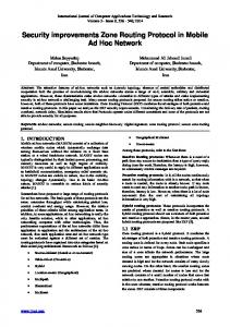
FIG. 1. 共a兲 The pheromone of links ij and ji. Generally, p ji ⫽ pij. 共b兲 The pheromone of a node is defined as the sum of pheromone of links going toward the node. For example, the pheromone of node b is pb = pab + pcb.

model: starting from m0 fully connected nodes, a new node with m 共m ⱕ m0兲 edges is added to the existing graph at each time step according to preferential attachment, i.e., the probability ⌸i of being connected to the existing node i is proportional to the degree ki of the existing node. In this paper, we set m0 = m = 5 and the network size N = 1000. The traffic model is described as follows. At each time step, there are R packets generated in the system, with randomly chosen sources and destinations. One node can deliver at most C 共in this paper we set C = 1兲 packets to its neighboring nodes. The packets are delivered by the local information of pheromone, which is defined on the links. In every time step, each node performs a local search among its neighbors. If a packet’s destination is found within the searched area, it is delivered directly to its target. Otherwise, the packet is delivered to a neighboring node j with probability Pi→j =

p␣ij

兺j p␣ij

,

共1兲

where pij is the pheromone of the link pointing from node i to node j, the sum runs over all neighbors of node i, and ␣ is a tunable parameter characterizing the routing preference. Note that pij can be different from p ji, as shown in Fig. 1共a兲. Once arriving at its destination, the packet will be removed from the system. The queue length of each node is assumed to be unlimited and the first in first out rule is applied to all queues. Next we introduce the updating rule for the pheromone of a link. Initially, the value of the pheromone concentration on each link is set to a small unit value of ␦ p. The pheromone of each link cannot be smaller than this value ␦ p. Whenever a packet is delivered successfully from node i to node j, the pheromone of link ij will be updated according to the following rule: if the queue length of node j is larger than a critical value, i.e., L j ⬎ Lc, the pheromone of link ij will decrease by a unit, pij = max兵pij − ␦ p, ␦ p其.

FIG. 2. 共Color online兲 Typical variation of N p for the pheromone routing strategy in the free-flow 共R ⬍ Rc兲 and jam 共R ⬎ Rc兲 states. The parameters are ␣ = 1.0 and ␤ = 2.0.

pij = pij + ␦ p.

In this paper, we set the unit value as ␦ p = 0.001. The critical queue length is set to be proportional to the delivery ability of the node: Lc = ␤C. Then we investigate the effects of ␣ and ␤ on the traffic dynamics of the system. III. SIMULATION RESULTS

In this section, we show the simulation results of the pheromone routing strategy on a BA scale-free network. Figure 2 shows the typical evolution of total packets number N p over time with the pheromone routing strategy. When R is smaller than a critical value Rc 共Rc characterizes the overall capacity of the system, which will be introduced later兲, one can see that the variation of N p can be divided into two stages: the relaxation and balanced stages. In the relaxation stage, N p first increases to a maximum and then decreases to a balanced state. In the balanced stage, N p is almost constant, indicating that the numbers of generated and removed packets are balanced. When R is larger than the critical value of Rc, N p increases to infinity, indicating that the system enters a jam state. In the relaxation stage, the concentration of pheromone is automatically adjusted to achieve an optimal state. One can investigate the normalized average node pheromone 具pk典 as a function of node degree k. A node’s pheromone is defined as the sum of the link pheromone going toward the node, as shown in Fig. 1共b兲. The normalized average node pheromone is calculated by Normalized 具pk典 =

具pk典 具pmax k 典

共4兲

,

with 具pk典 =

共2兲

Otherwise, if the queue length L j ⱕ Lc, the pheromone will increase by a unit value,

共3兲

⌺p共degree=k兲 Number 共degree = k兲

.

共5兲

Figure 3 shows the normalized pheromone 具pk典 for different evolution times for the system. In both the increasing and

066110-2

PHYSICAL REVIEW E 80, 066110 共2009兲

PHEROMONE ROUTING PROTOCOL ON A SCALE-FREE…

FIG. 3. 共Color online兲 The normalized average node pheromone 具pk典 at different times. Other parameters are R = 5, C = 1, ␣ = 1.0, and ␤ = 2.0.

decreasing periods of the relaxation stage 共T = 30 000 and 60 000兲, the normalized pheromone 具pk典 follows a power law. The average pheromone of low-degree nodes are higher than that of high-degree nodes. Because the hub nodes bear more traffic load, the node pheromone decreases according to Eq. 共2兲. On the other hand, in the balanced stage 共T = 300 000兲, the normalized pheromone 具pk典 is almost independent of k. At this point, the hub nodes have roughly the same pheromone as the low-degree nodes. Thus, the pheromone of the links going to hub nodes are much lower than that of the links going to low-degree nodes. According to the delivering rule, the packets are encouraged to go to lowdegree nodes. However, because the hub nodes have more links, the total delivering probabilities of going to hub nodes and low-degree nodes are similar. The ability of both hub nodes and low-degree nodes can be fully utilized. Thus, the system achieves its optimum. Figure 4 shows the relaxation stage of N p with different values of ␤. One can see that the behavior of N p is similar for

FIG. 4. 共Color online兲 The variation of N p with different ␤. The inset shows Tc with different ␤.

FIG. 5. 共Color online兲 共a兲 The order parameter ␩ as a function of generating rate R for pheromone routing strategy and local degree routing strategy. The routing parameter is set to ␣ = 1.0 for the pheromone routing strategy and ␣ = −1.0 for the local routing strategy. Other parameters are N = 1000, m0 = m = 5, C = 1, and ␤ = 2.0 for the pheromone routing strategy. 共b兲 Rc versus ␣ with constant node capacity C = 1. The maximum of Rc corresponds to ␣ = 1.0 marked by a dotted line.

different ␤. One important issue here is to figure out the optimal value of ␤, at which the relaxation stage will be shortest for the system. We can investigate the critical time Tc at which N p reaches the balanced stage. Figure 6 inset shows Tc with different values of ␤. When ␤ = 2, Tc reaches its minimum. Thus, we can see that ␤ = 2 is the optimum for the system to quickly reach the balanced state. In order to describe the phase transition of traffic flow in the network, we adopt the order parameter 关7兴 C 具⌬N p典 , t→⬁ R ⌬t

␩共R兲 = lim

共6兲

where ⌬N p = N p共t + ⌬t兲 − N p共t兲 and 具 ¯ 典 indicates the average over time windows of width ⌬t. In Fig. 5共a兲, the typical variation of ␩ against R is shown for the pheromone routing strategy and the local routing strategy. The pheromone routing strategy is with parameter ␣ = 1.0, at which we will demonstrate that the maximum overall capacity is achieved. The local routing strategy 关30兴 is with the parameter of ␣ = −1.0, at which the maximum capacity is reached. For R ⬍ Rc, ␩ remains at zero, indicating that the system is in the free-flow state. With the increase in packet generation rate R, there will be a critical value of Rc at which ␩ increases from zero, indicating that the packets accumulate in the system, and the system becomes seriously congested 关7兴. Therefore, Rc is the maximal generating rate under which the system can maintain its normal and efficient functioning. One can see that the pheromone routing strategy can reach a larger network capacity. As shown in Fig. 5共a兲, the maximal overall capacity is Rc = 3.7 with local degree routing strategy, while it is Rc = 5.3 for the local pheromone routing strategy. In Fig. 5共b兲, the overall capacity Rc is sought out for different values of routing parameter ␣ with constant node capacity C = 1. One can see that, when ␣ = 1.0, the system’s capacity can be enhanced maximally.

066110-3

PHYSICAL REVIEW E 80, 066110 共2009兲

LING et al.

FIG. 6. 共Color online兲 共a兲 Network capacity Rc vs average degree 具k典 with the same network size of N = 1000. 共b兲 Network capacity Rc vs network size N with the same average degree of 具k典 = 10. Other parameters are C = 1, ␣ = 1.0, and ␤ = 2.0 for both situations.

We also investigated the effects of average node degree 具k典 and network size N on the traffic capacity of network, as shown in Fig. 6. In Fig. 6共a兲, one can see that Rc increases almost linearly with the increase in average degree 具k典 and in Fig. 6共b兲, Rc also increase slightly with the increase in network size. To better understand why ␣ = 1.0 is the optimal value, we investigate the average packet number n共k兲 of nodes as a function of its degree k in the balanced stage, as shown in Fig. 7. The average is over the nodes with the same degree. When ␣ ⬍ 1.0 关Figs. 7共a兲 and 7共b兲兴, although the value of n共k兲 remains around 1.0, the distribution of n共k兲 follows a power law of n共k兲 ⬃ k␥ with exponent ␥ ⬎ 0. This indicates that the high-degree nodes are slightly overburdened. Since all nodes have the same delivering ability, this phenomenon will harm the system capacity. When ␣ = 1.0 关Fig. 7共c兲兴, n共k兲 is independent of k. The traffic load is homogeneously distributed among the nodes and thus lead to a maximum Rc.

FIG. 8. 共Color online兲 The probability distribution of traveling time for different ␣.

When ␣ ⬎ 1.0 关Fig. 7共d兲兴, there are obvious fluctuations in the value of n共k兲, especially for large-degree nodes. We also investigate the situations of bigger ␣ value. The fluctuations of n共k兲 are more evident. Therefore, it is easier for the hub nodes to get congested when ␣ ⬎ 1.0. So the system capacity decreases. Then we investigate the probability distribution of traveling time for different ␣ in a free-flow state. Packet traveling time is also an important factor for characterizing the network’s behavior. The traveling time is the time that a packet spends on traveling from a source to a destination. In Fig. 8, one can see that the distribution of traveling time follows a subpower law. Most packets can arrive at their destinations in a short time while some packets need to spend very long time to find their target nodes. We also note that, when ␣ = 1.0, the packets spend the shortest time for traveling. This is consistent with the result of Fig. 6 that the network’s capacity reached a maximum when ␣ = 1.0. Finally, we briefly introduce the effect of node delivering ability C on the traffic dynamics. The qualitative behavior is not affected by varying C. In general, the system’s overall capacity will increase with the increase in C, and the optimal value of ␣c remains the same. We also apply the pheromone routing strategy in ErdosRenyi and Watts-Strogatz networks 关1兴. The former provides a uniformly random reference, while the latter accounts for several types of real-world networks. However, the improvement in network capacity is not so obvious in these two networks. The pheromone routing strategy can perform better in a heterogeneous network than in a homogeneous network. IV. CONCLUSION AND DISCUSSION

FIG. 7. 共Color online兲 Average packet number for nodes n共k兲 depending on degree k for different ␣ in balanced stage. The error bars in 共d兲 show the fluctuations in the value of n共k兲. Other parameters are R = 3 ⬍ Rc, C = 1, and ␤ = 2.0.

In summary, we have proposed a routing protocol for a modern traffic system based on the local information of pheromone and then investigated the behavior of the traffic system. The system performs better under the pheromone routing strategy than under the local routing strategy by node degree or link bandwidth. Due to the difficulty of obtaining the information of the whole network’s topology in modern

066110-4

PHYSICAL REVIEW E 80, 066110 共2009兲

PHEROMONE ROUTING PROTOCOL ON A SCALE-FREE…

model can be useful for the design and optimization of routing strategies in some real traffic systems such as the urban transportation systems, peer-to-peer networks, wireless sensor networks, and so on.

communication and traffic systems, the routing protocols based on the local information are attracting much interest 关30–32兴. The pheromone routing strategy performs best among the routing protocols of local information. This is a nontrivial improvement in the network traffic area. In the model, the traffic system automatically adjust the distribution of pheromone to achieve a balanced state. In the balanced state, the traffic load will be homogeneously distributed among the nodes. The relaxation process depends on the traffic parameter. The optimal value of pheromone updating parameter ␤ should be set to ␤ = 2.0, at which the relaxation process will be minimal. Simulations have shown that the optimal routing strategy should be set to ␣ = 1.0, which is different from the local routing strategy 关30兴. The distribution of traveling time is also investigated. These phenomena are unique and can trigger more interest in this field. The

This work was funded by the National Basic Research Program of China 共Contract No. 2006CB705500兲, the NNSFC Key Project No. 10532060, Projects No. 70601026, No. 10672160, and No. 10872194, and the Innovation Foundation for Graduate Students of the University of Science and Technology of China under Grant No. W21103010012. R.W. and M.-B.H. acknowledge the support of Massey University International Visitor Research Fund.

关1兴 D. J. Watts and S. H. Strogatz, Nature 共London兲 393, 440 共1998兲. 关2兴 A.-L. Barabási and R. Albert, Science 286, 509 共1999兲. 关3兴 R. Albert and A.-L. Barabási, Rev. Mod. Phys. 74, 47 共2002兲. 关4兴 M. E. J. Newman, Phys. Rev. E 64, 016132 共2001兲. 关5兴 M. E. J. Newman, SIAM Rev. 45, 167 共2003兲. 关6兴 S. Boccaletti et al., Phys. Rep. 424, 175 共2006兲. 关7兴 A. Arenas, A. Díaz-Guilera, and R. Guimerá, Phys. Rev. Lett. 86, 3196 共2001兲. 关8兴 T. Ohira and R. Sawatari, Phys. Rev. E 58, 193 共1998兲. 关9兴 D. De Martino, L. Dall’Asta, G. Bianconi, and M. Marsili, Phys. Rev. E 79, 015101共R兲 共2009兲. 关10兴 R. V. Solé and S. Valverde, Physica A 289, 595 共2001兲. 关11兴 M. A. de Menezes and A.-L. Barabási, Phys. Rev. Lett. 92, 028701 共2004兲. 关12兴 S. Meloni, J. Gómez-Gardeñes, V. Latora, and Y. Moreno, Phys. Rev. Lett. 100, 208701 共2008兲. 关13兴 J. Duch and A. Arenas, Phys. Rev. Lett. 96, 218702 共2006兲. 关14兴 Z. Eisler, J. Kertesz, S.-H. Yook, and A.-L. Barabási, EPL 69, 664 共2005兲. 关15兴 Petter Holme and Beom Jun Kim, Phys. Rev. E 65, 066109 共2002兲. 关16兴 L. Zhao, K. Park, and Y. C. Lai, Phys. Rev. E 70, 035101共R兲 共2004兲. 关17兴 L. Zhao, Y.-C. Lai, K. Park, and N. Ye, Phys. Rev. E 71, 026125 共2005兲. 关18兴 R. Guimerà, A. Díaz-Guilera, F. Vega-Redondo, A. Cabrales, and A. Arenas, Phys. Rev. Lett. 89, 248701 共2002兲. 关19兴 R. Guimerà, A. Arenas, A. Díaz-Guilera, and F. Giralt, Phys. Rev. E 66, 026704 共2002兲. 关20兴 G. Yan, T. Zhou, B. Hu, Z. Q. Fu, and B. H. Wang, Phys. Rev. E 73, 046108 共2006兲. 关21兴 B. Danila, Y. Yu, J. A. Marsh, and K. E. Bassler, Phys. Rev. E

74, 046106 共2006兲. 关22兴 X. Ling, R. Jiang, X. Wang, M. B. Hu, and Q. S. Wu, Physica A 387, 4709 共2008兲. 关23兴 J. M. Kleinberg, Nature 共London兲 406, 845 共2000兲. 关24兴 B. J. Kim, C. N. Yoon, S. K. Han, and H. Jeong, Phys. Rev. E 65, 027103 共2002兲. 关25兴 L. A. Adamic, R. M. Lukose, A. R. Puniyani, and B. A. Huberman, Phys. Rev. E 64, 046135 共2001兲. 关26兴 Carlos P. Herrero, Phys. Rev. E 71, 016103 共2005兲. 关27兴 Shi-Jie Yang, Phys. Rev. E 71, 016107 共2005兲. 关28兴 B. Tadić, S. Thurner, and G. J. Rodgers, Phys. Rev. E 69, 036102 共2004兲. 关29兴 A. T. Lawniczak and X. Tang, Eur. Phys. J. B 50, 231 共2006兲. 关30兴 W. X. Wang, B. H. Wang, C. Y. Yin, Y. B. Xie, and T. Zhou, Phys. Rev. E 73, 026111 共2006兲. 关31兴 C. Y. Yin, B. H. Wang, W. X. Wang, T. Zhou, and H. Yang, Phys. Lett. A 351, 220 共2006兲. 关32兴 M. B. Hu, W. X. Wang, R. Jiang, Q. S. Wu, and Y. H. Wu, EPL 79, 14003 共2007兲. 关33兴 J. A. Pimentel, M. Aldana, Cristián Huepe, and Hernán Larralde, Phys. Rev. E 77, 061138 共2008兲. 关34兴 K. Nishinari, D. Chowdhury, and A. Schadschneider, Phys. Rev. E 67, 036120 共2003兲. 关35兴 A. John, A. Schadschneider, D. Chowdhury, and K. Nishinari, Phys. Rev. Lett. 102, 108001 共2009兲. 关36兴 A. Colorni, M. Dorigo, and V. Maniezzo, in Proceedings of the First European Conference on Artificial Life, Paris, 1991, edited by F. Varela and P. Bourgine 共Elsevier, Paris, 1991兲, pp. 134–142. 关37兴 L. da Fontoura Costa, F. A. Rodrigues, and G. Travieso, Phys. Rev. E 76, 046106 共2007兲. 关38兴 E. Bonabeau, M. Dorigo, and G. Theraulaz, Nature 共London兲 406, 39 共2000兲.

ACKNOWLEDGMENTS

066110-5