Pilot Beam Sequence Design for Channel Estimation in Millimeter ...

Pilot Beam Sequence Design for Channel Estimation in Millimeter-Wave MIMO Systems: A POMDP Framework

arXiv:1409.8434v1 [cs.IT] 30 Sep 2014

Junyeong Seo, Student Member, IEEE, Youngchul Sung, Senior Member, IEEE Gilwon Lee, and Donggun Kim, Student Members, IEEE

Abstract—In this paper, adaptive pilot beam sequence design for channel estimation in large millimeter-wave (mmWave) MIMO systems is considered. By exploiting the sparsity of mmWave MIMO channels with the virtual channel representation and imposing a Markovian random walk assumption on the physical movement of the line-of-sight (LOS) and reflection clusters, it is shown that the sparse channel estimation problem in large mmWave MIMO systems reduces to a sequential detection problem that finds the locations and values of the non-zerovalued bins in a two-dimensional rectangular grid, and the optimal adaptive pilot design problem can be cast into the framework of a partially observable Markov decision process (POMDP). Under the POMDP framework, an optimal adaptive pilot beam sequence design method is obtained to maximize the accumulated transmission data rate for a given period of time. Numerical results are provided to validate our pilot signal design method and they show that the proposed method yields good performance. Index Terms—Millimeter-wave, Large MIMO, Channel estimation, Partially Observable Markov Processes (POMDP)

I. I NTRODUCTION Millimeter-wave (mmWave) communication is rising as a key technology to provide high data rates with wide bandwidth (BW) in future wireless systems. However, the signal pathloss in the mmWave band is much larger than that in the lower band currently used in most wireless access networks. To overcome the pathloss, there is on-going research about highly directional beamforming techniques in mmWave systems using large antenna arrays [1]–[3]. Typically these beamforming techniques require channel state information (CSI) at the transmitter and the receiver, but it is more difficult to obtain CSI in the mmWave band than in the lower band because of the high propagation directivity and the low signal-to-noise ratio (SNR) before beamforming. Thus, the accurate and efficient channel estimation is important to attain the promised BW gain of the mmWave band. One of the major differences between the channels in conventional MIMO systems in lower bands and large mmWave MIMO systems is the sparsity in the MIMO channel. Whereas channel estimation methods in conventional lowerband MIMO systems assume rich scattering or the knowledge of the channel covariance matrix in the rank-deficient case, such assumptions are not valid in the mmWave band [4]. The authors are with the Dept. of Electrical Engineering, KAIST, Daejeon 305-701, South Korea. E-mail:{jyseo@, ysung@ee., gwlee@, and dg.kim@}kaist.ac.kr. This work was supported by ICT R&D program of MSIP/IITP [ 11-911-04-001, Development of Adaptive Beam Multiple Access Technology without Interference based on Antenna Node Grouping].

Among many possible ray directions resolved by a large antenna array, only a few directions actually carry the signal, and these signal-carrying directions are unknown beforehand [4]. To tackle the challenge of the sparse channel estimation in the mmWave band, algorithms based on compressed sensing (CS) have recently developed [2]–[5]. In [4], the channel estimation problem is formulated by capturing the sparse nature of the channel, and CS techniques are used to analyze the sparse channel estimation performance. Recently, an efficient channel estimation and training beam design method for large mmWave MIMO systems was proposed based on adaptive CS in [2], [3]. In the proposed method, the channel estimation is conducted over multiple slots under the assumption that the channel does not vary over the considered multiple slots. Each slot consists of multiple training beam symbol times so that the sparse recovery is feasible at each slot, and the training beam at the next slot is adaptively designed depending on the previous slot observation based on a space bisection approach [2], [3]. Such a design strategy is a reasonable choice to search the actual signal-carrying directions in the space. In this paper, we consider the adaptive pilot beam sequence design to estimate the sparse channel in large mmWave MIMO systems based on a decision-theoretical approach, and propose a strategy to design the pilot beam sequence that is optimal in a certain sense. Exploiting the sparsity of mmWave channels with the virtual channel representation and imposing a Markovian random walk assumption on the physical movement of the LOS and reflection clusters, we cast the sparse channel estimation problem in large mmWave MIMO systems into the framework of a partially observable Markov decision process (POMDP) with finite horizon [6], where we need to find the locations and values of the non-zero-valued bins in a twodimensional rectangular grid. Under the proposed POMDP framework, we derive an optimal adaptive pilot beam sequence design method to maximize the accumulated transmission data rate for a given period of time. II. S YSTEM M ODEL A. Sparse Channel Modeling in mmWave Systems We consider a mmWave MIMO system with a uniform linear array (ULA) of Nt antennas at the transmitter and an ULA of Nr antennas at the receiver. The received signal at symbol time n is given by yn = Hn xn + nn , n = 1, 2, · · · ,

(1)

where Hn is the Nr × Nt MIMO channel matrix at time n, xn is the Nt × 1 transmitted symbol vector at time n with a power constraint E{xn xH n } ≤ Pt , and nn is the Nr × 1 2 Gaussian noise vector at time n from CN (0, σN INr ). The MIMO channel matrix Hn can be expressed in terms of the physical propagation paths as Hn =

L X p r t Nt Nr αn,ℓ aRX (θn,ℓ )aH T X (θn,ℓ ),

(2)

ℓ=1

where αn,ℓ ∼ CN (0, ξ 2 ) is the complex gain of the ℓ-th r t path at time n, and θn,ℓ and θn,ℓ are the angle-of-arrival (AoA) and angle-of-departure (AoD) normalized directions of the ℓ-th path at time n for the receiver and the transmitter, respectively. Here, the normalized direction θ is related to the , where d is physical angle φ ∈ [−π/2, π/2] as θ = d sin(φ) λ the spacing between two adjacent antennas and λ is the signal wavelength (we assume λd = 12 ), and aRX (θr ) and aT X (θt ) are the receiver response and the transmitter steering vector, which are defined as [7] r r 1 aRX (θr ) = √ [1, e−ι2πθ , · · · , e−ι(Nr −1)2πθ ]T , Nr t t 1 aT X (θt ) = √ [1, e−ι2πθ , · · · , e−ι(Nt −1)2πθ ]T . Nt

(3) (4)

With neglecting the angle quantization error the physical MIMO channel matrix Hn can be rewritten in terms of the virtual channel matrix HVn [8]: Hn = AR HVn AH T ,

(5)

r where AR = [aRX (θ˜1r ), · · · , aRX (θ˜N )], θ˜ir = − 21 + i−1 Nr for r t t i = 1, · · · , Nr , and AT = [aT X (θ˜1 ), · · · , aT X (θ˜N )], θ˜jt = t j−1 − 21 + Nt for j = 1, · · · , Nt . The element in the i-th row and the j-th column of HVn indicates the complex channel gain whose AoA and AoD normalized directions are θ˜r,i and θ˜t,j , respectively. The sparsity in the physical channel model in (2) is translated into Nt X j=1

||HVn (:, j)||0 = L,

To design a very efficient pilot beam sequence, we exploit the channel dynamic, and model the channel dynamic by using a Markovian structure that is different from the Gauss-Markov or state-space channel model conventionally used to model the channel dynamic. In large mmWave MIMO systems, the sparsity should be captured in the channel dynamic. Here, we focus on the locations of the non-zero elements of HVn rather than the values, since the value will be obtained with reasonable quality once the correct direction is hit by the pilot beam with high power. Note that each propagation path is generated by either LOS or a reflection cluster and the physical movement of the receiver or a reflection cluster can be modelled as a random walk in space. This random walk translates into each nonzero bin’s random walk in the virtual channel matrix. Thus, we assume a stationary block Markovian random walk for the dynamic of the virtual channel matrix. That is, the virtual channel matrix HV(k) at slot k is constant over the slot and changes to HV(k+1) at the next slot k + 1 with the aforementioned random walk with a set of transition probabilities. We also assume that the movement of each path is independent. Since the receiver checks all possible AoA directions in parallel, we here only consider the random walk across AoD, i.e., the column-wise movement of each non-zero bin in the virtual channel matrix. 1) The Single Path Case: First, consider the single path case, i.e., L = 1. The single path (or non-zero bin) is located in a certain column of the virtual channel matrix at slot k, and stay at the same column or moves to another column of the virtual channel matrix at slot k + 1 according to the explained random walk. Since we have Nt columns in the virtual channel matrix, the number N of states for L = 1 is Nt . Let us denote the set of all possible states by S given by S = {1, 2, · · · , Nt }, where state i denotes the state that the path is located in the i-th column of the virtual channel matrix. With the set S of states defined, the (i, j)-th element of the N × N state transition probability matrix P is given by pij = Pr{Sk+1 = j|Sk = i}, i, j ∈ S,

where L ≪ Nt Nr for large Nt . We assume that the receiver has Nr (≪ Nt ) RF chains so that it can implement the filter bank AH R to look ahead for all possible AoA directions. In this case, the receiver filter-bank output is given by V H ′ yn′ := AH R yn = Hn AT xn + nn

B. The Proposed Dynamic Channel Model

(6)

where n′n = AH R nn . By simply transmitting a pilot beam sequence aT X (θ˜1t ), t aT X (θ˜2t ), · · · , aT X (θ˜N ), the receiver can estimate the pot sitions and values of the L non-zero elements of HVn if the channel is time-invariant for Nt symbol times. However, such a method does not exploit the channel sparsity and/or the channel dynamic, and is inefficient when Nt is large.

(7)

where Sk and Sk+1 denote the states of slots k and k + 1, respectively. The transition probability matrix captures the characteristics of the path’s movement behavior and thus it should carefully be designed by considering the physics of the receiver and reflection cluster movement, e.g., vehicular channels or pedestrian channels. Intuitively, it is reasonable to model P such that the transition probability from column i to column j is monotonically decreasing with respect to (w.r.t.) |i − j|. That is, it is more likely to shift to a nearby column. In the extreme case of a static channel, we have P = I. If we ignore the possibility of the path’s movement with a large AoD change, we can model the transition probability matrix as a banded matrix. For the example of Nt = 5, one way to model the transition probability matrix is given by

0.5

at time k = 1

at time k = 2

0.5

Feedback

State transition slot (k + 1)

˜r } (AoA) {θ m

˜r } (AoA) {θ m

slot (k) α1,1 α1,2

Data transmission

α2,2 α2,1

Mp

Data transmission · · · Mp

A sequence of pilot beams for Mp symbol times aT X (θ˜itMp ) ··· aT X (θ˜it1 ) aT X (θ˜it2 ) ˜t } (AoD) {θ n

−0.5

0.5

˜t } (AoD) {θ n

−0.5

0.5

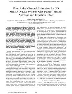
Fig. 1. An illustration of a transition of each path when L = 2 and Nt = Nr = 7.



   PB β = 

P 1 − 2i=1 αβ i P2 1 − i=0 αβ i αβ 2 0 0

αβ α αβ αβ 2 0

αβ 2 αβ α αβ αβ 2

0 αβ 2 αβ α αβ

0 0 αβ 2 P 1 − 2i=0 αβ i P 1 − 2i=1 αβ i



  ,   (8)

where β is a decreasing factor that captures the amount of probability reduction w.r.t. the column distance, and α is the value that makes the sum of each row in (8) one. 2) The Multiple Path Case: Now consider the multiple propagation path case, i.e., L ≥ 2. In this case, each path (or non-zero bin) is located in a column of the virtual channel matrix. The set S of all possible states is now given by S = {(i1 , i2 , · · · , iL ), i1 , i2 , · · · , iL = 1, 2, · · · , Nt },

(9)

where state (i1 , · · · , iℓ , · · · , iL ) denotes that the ℓ-th path is located at the iℓ -th column of the virtual channel matrix for ℓ = 1, · · · , L and the cardinality N of S is NtL . For notational simplicity, let us also use the following notation: S = {s(1) , s(2) , · · · , s(N ) },

(10)

where states (i1 , · · · , iL ), i1 , · · · , iL = 1, · · · , Nt , are enumerated into states s(i) , i = 1, 2, · · · , N = NtL . We here allow multiple paths can merge on and diverge from a column of the virtual matrix. Then the state transition probability in the L independent path case is given by Pr{Sk+1 = (j1 , · · · , jL )|Sk = (i1 , · · · , iL )} = pi1 j1 pi2 j2 × · · · × piL jL ,

(11)

where pij denotes the transition probability that a path moves from the i-th column to the j-th column of the virtual channel matrix at the next slot and is defined in (7). Fig. 1 illustrates an example of transitions of the paths when L = 2 and Nt = Nr = 7. The transition probability of Fig. 1 is p67 × p24 due to the independence assumption for each path. C. Channel Sensing with Pilot Beams We assume that Mp (L ≤ Mp ≪ Nt ) symbol times in each slot are used for transmitting a sequence of pilot beams and one column of AT is selected as the pilot beam in each pilot

Fig. 2.

The process of the pilot training.

symbol time. (We assume that highly directional pilot beam is required to obtain a channel gain estimate with reasonable quality due to large pathloss in the mmWave band.) Hence, Mp columns of AT are selected as the pilot beam sequence for the Mp pilot symbol times per slot. If aT X (θ˜itm ) is transmitted as the pilot signal at the m-th pilot symbol time in the k-th slot, from (6), the receiver filter-bank output is given by ′ y(k) [m] = HV(k) (:, im ) + n′(k) [m],

(12)

′ where y(k) [m] denotes the receiver filter-bank output at symbol time m of slot k, n′(k) [m] is similarly defined, and HV(k) (:, im ) denotes the im -th column of HV(k) . After the transmission of the sequence of pilot beams for one slot is finished, the receiver senses and estimates the Mp columns of HV(k) corresponding to the Mp pilot beams. Then, the receiver feedbacks the sensing results and estimated channel gains corresponding to the Mp pilot beam directions to the transmitter. The process is depicted in Fig. 2. Now, the problem is to design the sequence of pilot beams for Mp symbol times for each slot in a certain optimal way. Since Mp ≪ Nt , we can only sense a few columns of HV(k) at slot k. Therefore, Mp pilot beams at each slot should be designed judiciously by exploiting the channel dynamic and the available information in all the previous slots.

III. POMDP F ORMULATION FOR P ILOT B EAM D ESIGN FOR S PARSE C HANNEL E STIMATION A. Action Space at the Transmitter and Feedback from the Receiver In Section II, we assumed that Mp columns of AT are selected as the pilot beam sequence for the Mp pilot symbols per slot. This is equivalent to choose Mp columns of the virtual channel matrix at each slot to be sensed by the pilot beam sequence. We denote the selected column indices of the virtual channel matrix by a = [a1 , a2 , · · · , aMp ], where am indicates the index of the column of the virtual channel matrix that is sensed at symbol time m.
(a is referred Nt possible a’s to as the action vector.) Hence, there are M p and the optimal pilot beam sequence design problem reduces to choosing the best a at each slot. After the chosen pilot beam sequence is transmitted to the receiver, the receiver feedbacks the result of detection

State transition

Pilot beam Feedback selection observation a

P

o

C. The Reward and The Policy

Reward rk (s, a, o)

slot k π k+1

πk Fig. 3.

The sequence of operation at slot k

to the transmitter for pilot beam sequence design for the next slot. The feedback information contains the information about the existence∗ of paths in the selected columns of the virtual channel matrix as well as the complex gains of the detected paths. Then, the transmitter uses the channel gain information of the detected paths for beamforming during the data transmission period and uses the feedback information about the existence of paths to choose the pilot beam sequence for the next slot in an adaptive manner. The latter feedback information can be modeled as o = [o1 , o2 , · · · , oMp ] ∈ {0, 1}

Mp

,

(13)

where om = 1 indicates that a path is detected by the pilot beam transmitted at the m-th pilot symbol time, and otherwise om = 0. Since there exist 2Mp possibilities in o, the feedback Mp information space is defined as O = [o(1) , o(2) , · · · , o(2 ) ]. When the current state of the virtual channel matrix is s(i) and the action vector a is selected for the pilot beam sequence for the current slot, the probability that the transmitter observes a the feedback information o(j) is denoted as qij , i.e., a qij , Pr{o = o(j) |s(i) , a}

for s(i) ∈ S, o(j) ∈ O.

(14)

This probability depends on the detector used to identify the existence of a non-zero bin in a column at the receiver. B. Sufficient Statistic Fig. 3 describes the sequence of the operation at slot k consisting of the current belief vector πk , state transition, action, observation, and reward. At the beginning of slot k, the information from all the past slot pilot beam sequences and feedback information can be summarized as a belief vector:† π k = [πk,1 , πk,2 , · · · , πk,N ],

(15)

where πk,i is the probability that the state at the beginning of slot k is state s(i) conditioned on all past pilot beam sequences and feedback information. It is known that the belief vector is a sufficient statistic for the action, i.e., the design of the optimal pilot beam sequence for slot k [9]. The transmitter uses the belief vector to optimally choose the action, i.e., the pilot beam sequence for slot k that maximizes the expected reward, and updates the belief vector for the next block based on new feedback information. ∗ The detection can be wrong. This is another reason for POMDP in addition to the limited search of Mp columns out of the Nt total columns per slot. † Note that the belief vector π is conventionally defined prior to the state k transition for each slot, as shown in Fig. 3. The belief vector after the state transition can simply be updated by using the state transition probability matrix.

A reward is gained during the data transmission period according to the accuracy of channel estimation. According to the objective, there can be several ways to define the reward. Since we want to track all actual propagation paths in the sparse mmWave MIMO channel successfully, we define the reward for each slot as the number‡ of actual propagation paths (i.e., the number of non-zero bins in the virtual channel matrix) detected by the selected pilot beam sequence. If the state of the virtual channel matrix at slot k is s(i) , the selected pilot beam sequence or the action vector at slot k is a, and the transmitter observes the feedback information o(j) , then the immediate reward at slot k is expressed as Mp X

r(s(i) , a, o(j) ) =

(j) NsBIN (i) ,a om m

(16)

m=1

is the number of non-zero bins in column am where NsBIN (i) ,a m (j)

when the virtual channel matrix is in state s(i) , and om is the m-th element of o(j) . (Two paths with the same AoD and different AoAs are considered as two different paths.) Here, the false alarm of the receiver detector does not affect the (j) = immediate reward because in this case om = 1 but NsBIN (i) ,a m 0. In the case of miss detection, the opportunity is simply lost. Since the state at slot k and the feedback information are unknown at the time of action, we should consider the expected reward [6]. If the state of the virtual channel matrix prior to the state transition at slot k is s(n) , then the immediate expected reward at slot k is R(s(n) , a) =

N X

pni

j=1

i=1

=

N X

Mp 2 X

pni

i=1

Mp 2 X

j=1

Pr{o = o(j) |s(i) , a}r(s(i) , a, o(j) ) a qij

Mp X

(j) NsBIN (i) ,a om , m

(17)

m=1

where the state transitionPfrom s(n) to all possible s(i) within N the slot is captured by i=1 pni (·). When the belief vector π k is given at the beginning of slot k and Sk is the random variable representing the state at the beginning of the slot, the immediate expected reward at slot k is given by R(π k , a) = =

E{R(Sk , a)|π k } hR(a), π k i

(18)

where R(a) = [R(s(1) , a), R(s(2) , a), · · · , R(s(N ) , a)], and h·, ·i denotes the inner product operation. In the POMDP framework, a policy δ is defined as a sequence of functions that maps the belief vector to an action i.i.d.

‡ With α ∼ CN (0, ξ 2 ) in (2), the data rate will roughly be (k),l log(1 + Np ξ 2 ) in case of maximal ratio combining (MRC) transmission or Np log(1 + ξ 2 ) in case of spatial multiplexing used at the transmitter, where Np is the number of identified paths. Thus, Np directly captures the data rate for the case of spatial multiplexing. In case of MRC transmission, log(1 + Np ξ 2 ) can be used as the reward without change in the formulation.

for each slot [9], [10], where the action in our formulation is the choice of the pilot beam sequence. The optimal policy is the policy that maximizes the total immediate expected reward over T slots§ when the initial belief vector π 1 at the beginning of the transmission is given. In other words, the optimal policy δ ∗ is expressed as " T # X ∗ (19) δ = arg max Eδ R(Sk , ak )|π 1 , δ

k=1

where ak is the action vector at slot k, Eδ is the conditional expectation when the policy δ is given, and T is the total number of slots. IV. T HE O PTIMAL AND S UBOPTIMAL S TRATEGIES FOR C HANNEL E STIMATION Under the proposed formulation the optimal pilot beam sequence design problem is equivalent to the problem of finding the optimal policy that satisfies (19). When the initial belief vector π 1 is given at k = 1, we can define an optimal value function V (π 1 ) as the maximum total expected reward by the optimal policy δ ∗ : " T # X (20) R(Sk , ak )|π 1 . V (π 1 ) = Eδ∗ k=1

Now consider V k (π k ) defined as the maximum remaining expected reward that can be obtained from slot k to slot T when a belief vector πk is given at the beginning of slot k. Then, V k (π k ) can be decomposed as [11] V k (π k )   Mp 2X   k+1 (j) (j) = max hR(ak ), π k i + V (T (π k |o , ak ))γ(o |πk , ak ) , ak   j=1

(21)

PN ak PN where γ(o(j) |π k , ak ) = i=1 qij n=1 πk,n pni and T (π k |o(j) , ak ) is the updated belief vector from π k at slot k for the next slot after taking action ak and observing o(j) . T (π k |o(j) , ak ) can easily be computed using Bayes’s formula as [9], [10] π k+1 = [πk+1,1 , πk+1,2 , · · · , πk+1,N ] = T (π k |o(j) , ak ), where the i-th element of π k+1 is given by πk+1,i = Pr{sk = s(i) |o(j) , ak , π k } ak PN qij n=1 πk,n pni = PN a PN . k i=1 qij n=1 πk,n pni

(22)

The optimal policy δ ∗ over the considered transmission period k = [1, 2, · · · , T ] can be computed via the recursion (21) from backward once the state transition probability P, reward, and observation and action spaces are given [9], [10], [12]. This computation can be done off-line and the optimal § Such

a formulation is called a finite-horizon POMDP. The formulation here can be modified to the infinite-horizon case.

policy can be stored beforehand.¶ Then, in actual transmission, we start from k = 1 with π 1 and repeat action and observation. The complexity of this actual operation is insignificant. As the number of states and the size of the action space increase, obtaining the optimal policy for the POMDP problem requires high complexity. To reduce the computational complexity, we can use point-based POMDP value iteration algorithms proposed in [13]–[15]. Alternatively, to reduce the complexity, we can simply use the greedy policy that considers only the immediate expected reward at each slot. V. N UMERICAL

RESULTS

In this section, we provide some numerical results to evaluate the performance of the proposed pilot beam design and channel estimation for sparse mmWave MIMO channels. Throughout the simulation, we fixed the number of paths in the MIMO channel as L = 2 and assume that each path moves independently. The receiver uses the ML detector for sensing the paths and the noise power at the receiver side is 2 σN = 1 and the transmit power is fixed to 1 dB higher than the noise power before beamforming. (After beamforming with Nt transmit antennas, the SNR increases correspondingly.) We first considered the MIMO channel with Nt = 8 transmit antennas and Nr = 4 receive antennas. We set Mp = 4 and used PB β in (8) with bandwidth 1 for each path’s movement. Fig. 4 shows the performance of the optimal POMDP strategy, the greedy POMDP strategy and a random beam selection strategy, where the y-axis in the figure indicates the slot reward averaged over 100, 000 MIMO channel process realizations. Fig. 4 (a) shows the performance when the initial state information is unknown so that all the elements of the initial belief vector are set to be equal, and Fig. 4 (b) shows the performance when the initial state information is perfectly known. Thus, we can consider that Fig. 4 (a) shows the initial transient behavior whereas Fig. 4 (b) shows the steady-state tracking behavior. In the random pilot beam
Nt possible pilot beam sequences selection strategy, one of M p is randomly selected to sense the channel at each slot. It is shown in Fig. 4 that the optimal POMDP strategy and the greedy PODMP strategy significantly outperform the random pilot beam selection strategy. It is also shown in the figure that the performance gap between the optimal strategy and the greedy strategy is not significant in this case. Next, we considered a larger MIMO channel with Nt = 16 transmit antennas and Nr = 4 receive antennas. We set Mp = 6 and used PB β in (8) with bandwidth 2 for the channel dynamic. In the case, we focused on the tracking performance with the assumption of perfect knowledge of the initial state information to show the ineffectiveness of simple heuristic tracking strategies. In this case, the POMDP size is large and thus we considered the suboptimal greedy pilot beam design method only. Fig. 5 shows the performance of the greedy POMDP strategy, a heuristic strategy, and the random strategy. ¶ Hence, for each channel type, we can pre-compute the policy and store it. This is one of the main advantages of the proposed pilot beam design approach.

algorithm computes the most probable three columns for the next slot pilot beams based on the currently detected column and PB β . If no path is detected at the previous slot, the pilot beam indices do not change. It is seen that the greedy POMDP strategy yields better performance than the other strategies.

1.8 1.7

POMDP(optimal) POMDP(greedy) Random

β= 0.5

The averaged reward

1.6 1.5 β= 0.9

1.4

VI. C ONCLUSION

1.3 1.2 1.1 1 0.9 1

2

3

4

5

6

7

8

9

10

Block

(a) 1.8 POMDP (optimal) POMDP (greedy) Random

β = 0.5

1.7

The averaed reward

1.6 1.5 1.4

β = 0.9

We have considered the pilot beam sequence design for sparse large mmWave MIMO channels. We have shown that the pilot beam design problem can be formulated as a POMDP problem by exploiting the sparse channel dynamic and have obtained the optimal strategy and a greedy strategy for pilot beam sequence design. The proposed pilot design method can be used to estimate the channel initially at the beginning of the transmission or to track the channel once the sparse channel locations are identified with some other method. For the initial channel identification purpose, the proposed algorithm can be modified by considering a superposed pilot beam for a pilot symbol time with adaptive resolution over slots to shorten the time for initial path location identification.

1.3

R EFERENCES

1.2 1.1 1 0.9 1

2

3

4

5

6

7

8

9

10

Block

(b) Fig. 4. The performance of the optimal strategy and the greedy strategy in POMDP. (Nt = 8, Nr = 4, Mp = 4, L = 2)

50 45

Th accumulated reward

40 35

POMDP (greedy, β =0.5) Heuristic (β =0.5) Random (β =0.5) POMDP (greedy, β =0.9) Heuristic (β =0.9) Random (β =0.9)

30 25 20 15 10 5 0 0

5

10

15 Block

20

25

30

Fig. 5. The performance of the greedy strategy in POMDP, a heuristic tracking strategy in the MIMO channel, and the random selection strategy. (Nt = 16, Nr = 4, Mp = 6, L = 2),

The y-axis in Fig. 5 is the averaged accumulated reward to the point of the x-axis averaged over 10, 000 MIMO channel process realizations. In the heuristic tracking strategy, 3 pilot symbol times out of the total 6 pilot symbol times per slot are used to track one path and the other three symbol times are used to track the other path based on the detection result of the previous slot. If a path is detected at a certain column at the previous slot, the

[1] O. E. Ayach, R. W. Heath Jr., S. Abu-Surra, S. Rajagopal, and Z. Pi, “Low complexity precoding for large millimeter wave MIMO systems,” Proc. IEEE Int. Conf. Commun., Jun. 2012. [2] A. Alkhateeb, O. E. Ayach, G. Leus, and R. W. Heath, “Hybrid precoding for millimeter wae cellular systems with partial channel knowledge,” in Proc. Inf. Theory and Appl. Workshop., (San Diego, CA), 2013. [3] A. Alkhateeb, O. E. Ayach, G. Leus, and R. W. Heath, “Channel Estimation and Hybrid Precoding for Millimeter Wave Cellular Systems,” arXiv preprint arXiv:1401.7426., 2014. [4] W. U. Bajwa, J. Haupt, A. M. Sayeed, and R. Nowak, “Compressed channel sensing: a new approach to estimating sparse multipath channels,” Proc. IEEE., vol. 98, pp. 1058 – 1076, Jun. 2010. [5] G. Taub¨ock and F. Hlawatsch, “Compressed sensing based estimation of doubly selective channels using a sparsity-optimized basis expansion,” in Proc. Eur. Signal Process. Conf., (Switzerland), Aug. 2008. [6] M. L. Puterman, Markov decision processes: Discrete stochastic dynamic programming. John Wiley & Sons, 1994. [7] A. M. Sayeed and V. Raghavan, “Maximizing MIMO capacity in sparse multipath with reconfigurable antenna arrays,” IEEE J. Sel. Topics Signal Process., vol. 1, pp. 156 – 166, Jun. 2007. [8] A. M. Sayeed, “Deconstructing multiantenna fading channels,” IEEE Trans. Signal Process., vol. 50, pp. 2563 – 2579, Oct. 2002. [9] R. D. Smallwood and E. J. Sondik, “The optimal control of partially observable Markov processes over a finite horizon,” in Operations Research, vol. 21, pp. 1071–1088, 1973. [10] E. Monahan, “State of the ArtA Survey of Partially Observable Markov Decision Processes: Theory, Models, and Algorithms,” Management Science. , vol. 28, no. 1, pp. 1 – 16, 1982. [11] S. M. Ross, Applied probability models with optimization applications. Courier Dover Publications, 1970. [12] A. Cassandra, M. L. Littman and N. L. Zhang, “Incremental pruning: A simple, fast, exact method for partially observable Markov decision processes,” Proc. Thirteenth Ann. Conf. on Uncertainty in Artificial Intelligence., pp. 54 – 61, Morgan Kaufmann Publishers Inc., 1997. [13] J. Pineua, G. Gordon, and S. Thrun, “Point-based value iteration: An anytime algorithm for POMDPs,” in Proc. Int. Joint Conf. Artificial Intelligence, vol. 3, pp. 1025 – 1032, 2003. [14] H. Kurniawati and D.Hsu and W. Lee, “SARSOP: Efficient Point-Based POMDP Planning by Approximating Optimally Reachable Belief Spaces,” in Proc. Robot. Sci. Syst, 2008. [15] T. Smith and R. Simmons, “Point-based POMDP algorithms: Improved analysis and implementation,” arXiv preprint arXiv:1207.1412 , 2012.