channel height for congestion analysis in VLSI design automation. ... during early design stages. ..... [3] Naveed Sherwani, Algorithms for VLSI Physical Design.
CHANNEL HEIGHT ESTIMATION IN VLSI DESIGN Lun Li, Theodore W. Manikas
He Jin
Department of Electrical Engineering The University of Tulsa Tulsa, OK 74104
Department of Electrical and Computer Engineering Oklahoma State University Tulsa, OK 74106
ABSTRACT Abstract --This paper presents four methods to estimate channel height for congestion analysis in VLSI design automation. Our channel height estimation methods consider constraint graphs and net types in a channel. The experimental results show that the proposed methods yield better results than existing methods.
is not accurate for channel height estimation. In this paper, four methods have been proposed to estimate channel height.
h = ts × TT + TB + Max( LT , LB )
Top terminals
1. INTRODUCTION As the VLSI technology advances, millions of transistors can be packed onto the surface of a chip. Unfortunately, the increased circuit density also introduces additional congestion. Intuitively speaking, congestion in a layout means too many nets are routed in local regions. This causes detoured nets and unroutable nets in detailed routing. Congestion deteriorates design performance because the detoured nets increase wirelengths and delays. Unroutable nets increase the time to market and expense [3]. Therefore, estimation algorithms are required for congestion analysis during early design stages. In recent years, several congestion estimation and removal methods have been proposed. They fall into two categories: congestion estimation and removal during global routing stage [6,12], and congestion estimation and removal during placement stage [5,7,8,9,10,11,13,14,15]. The congestionbased global routers reduce congestion through balancing the routing density of the channels involved with a given router. However, methods performed during the global routing stage are unlikely to achieve optimality because the net locations are already fixed at this stage [10]. There are several state-of-the-art congestion estimation methods in placement stage. However, most of them ignore the height of channels when they estimate the demand of routing resources [16]. Channel routing is the most common part of detailed routing for standard cells. Ignorance of channel height causes inaccurate estimation of congestion. Upton proposed a method to estimate channel height in [1]. Assume that LT , LB are the lengths of the top and bottom boundary
(1)
Channel
Top boundary LT
h
Bottom bounbary
Bottom terminals
LB
Figure 1 A channel in a layout
2. PROBLEM FORMULATION A given channel routing problem is specified by channel length, top and bottom terminal list, left and right connection list, and the number of layers [16]. The channel length is specified in terms of number of columns in grid-based models [3].
2.1 Net types There are three types of nets in a channel, as shown in Figure 2. Type 1 nets, N T , are nets that start and end in the channel. Type 2 nets are nets that have at least one terminal in the channel but have right and/or left connections T ype 2 N et
T y p e 1 N e ts
0
1
4
5
1
6
7
0
4
9
10
10
2
3
5
3
5
2
6
8
9
8
7
9
of the channel respectively, as shown in Figure 1; and TT , TB are the number of terminals on the top and bottom boundary of the channel respectively. The estimated channel height of [1] is shown as Equation 1. However, this method
T y p e 3 N e ts
T ype 2 N et
Figure 2 Net types
with the other blocks, N R and N L are the left and right
terminal belongs to N j and i ≠ j . Given a channel routing
connection nets respectively. Type 3 nets, N S , are pass
problem, a vertical constraint graph (VCG), is a directed graph Gv = (V , E v ) [3] where
through nets that have no connections in the channel. The total number of nets in a channel is N .
2.2 Constraint graphs There are two constraints for the type 1 and type 2 nets in a channel: horizontal constraint and vertical constraint.
2.2.1 Horizontal Constraint There is a horizontal constraint between two nets if these two nets will overlap each other when placed on the same track. Given a channel routing problem, a horizontal constraint graph (HCG), is a undirected graph Gh = (V , E h ) [3] where
v = { vi | vi represents I i corresponding to N i } E k ={( vi , v j )| I i and I j have a non-empty intersection} Figure 3 shows a channel and its HCG, e.g. net 1 and net 3 has horizontal constraint. The HCG plays a major role in determining the channel height. In a grid-based two-layer model, no two nets that have a horizontal constraint may be assigned to the same track [2]. 0
1
4
5
1
6
7
0
4
0
2
3
5
3
5
2
6
7
0
2
8
8
Ev ={( vi , v j )| N i has a vertical constraint with N j } Figure 4 shows the VCG for the channel in Figure 2, e.g. net 1 has vertical constraint with net 5. VCG also plays an important role in determining the channel height. In a gridbased two-layer model, no two nets in a directed path may be routed in the same track if doglegs are not allowed [2]. Let hmax and v max represent the maximum clique in the HCG and the longest path in VCG respectively for a channel. 1
4
8
5
7
3
6
L o ng est p a th
2
Figure 4 VCG for a channel Theorem 1 The lower bound on the number of tracks of a two-layer dogleg free routing problem is max { hmax , v max } [3].
3. PROPOSED METHODS 0
M axim um Clique
1
3
7
2
The proposed methods are based on the three net types in the channel and constraint graphs.
3.1 Method 1: Constraint Graphs with Actual Pass Through Nets In method 1, type 1 and type 2 nets are estimated using constraint graphs. The estimation equation is
5
6
4
7 8
Figure 3 A channel and its HCG
2.2.2 Vertical Constraint A net N i , in a grid-based model, has a vertical constraint with net N j if there exists a column such that the top terminal of the column belongs to N i and the bottom
he1, 2 = Max { hmax , v max }
(1)
Where he1, 2 is the estimated channel height for type 1 and 2 nets Type 3 nets, N s , are the nets that pass through the channel but are not connected to modules adjacent to the channel. One pass through net will occupy one whole track in the final detailed routing solution. The number of pass through nets, N s , is determined in global routing stage. We use the actual number of pass through nets in method 1. The total estimated channel height is
he = ts × (he1, 2 + N s )
(2)
Where ts is the track spacing of the design rules, he is the total estimated channel height. 3.2 Method 2: Constraint Graphs with Estimated
Pass Through Nets In method 2, we use the same estimation method for type 1 and type 2 nets as method 1. We try to find a way to estimate type 3 nets. According to [1], the longer the channel, the more likely that nets will pass through it. Thus we could use the channel length to estimate the number of type 3 nets in placement stage. LT is the length of the top boundary, where LB is the length of the bottom boundary. he3 is the estimated height number of type 3 nets and the equation is
he3 = Max( LT , LB )
(4)
3.3 Method 3: HCG with Estimated Pass Through Nets From experimental results, we found that HCG is more important in determining channel height than VCG, and it takes less time to construct HCG than VCG. In method 3, we use hmax to estimate type 1 and type 2 nets. The estimation for type 3 nets is same as method 2. The final estimation equation is he = ts × h max + Max( LT , L B )
(5)
3.4 Method 4: Another Improved Method In method 4, we consider the right (left) connection list instead of the constraint graphs. All right (left) connection nets will pass the right (left) end column of the channel. According to the HCG, one right connection net should occupy one track in right end column of channel; one left connection net should occupy one track in left end column of channel. We have the following equation: The minimum channel height ≥ Max ( N R , N L )
he1, 2 = Max( N L , N R ) + N − N R − N L
(6)
So the number of right (left) connection nets needs to be considered in estimation. The channel was divided into two types. A type 1 channel is a channel where
N < Max ( N R , N L ). A type 2 channel is
a channel where
N > Max ( N R , N L ).
(7)
We use the same method for type 3 nets as method 2. So the final estimation equation for type 1 channels is he = ts × ((Max( N L ,N R ) + N − N R − N L ) + Max( LT ,LB ) (8)
For type 2 channels, we use terminals instead of nets in the channel to estimate type 1 nets. We use the same method for type 3 nets as method 2. Thus the final estimation equation for type 2 channel is he = ts × ( Max( N L , N R ) + TT + T B ) + Max ( LT , L B )
(3)
Incorporating the estimation for type 1 and type 2 nets in method 1, the final estimation equation is he = ts × he1, 2 + Max( LT , L B )
For type 1 channels, there exist a large number of right (left) connection nets. Considering Equation 6, we estimate channel height for type 1 and type 2 nets by the following equation:
(9)
4. RESULTS We tested our four proposed methods and Upton’s method on 12 benchmarks, Ex1, 2, 7–12 from [2] and Ex3–6 from [4]. The results are shown as Table 1. We define Average Estimation Error (AEE) as n E i − Ti e=
∑ i =1
Ti n
×100%
(10)
Where: n is the number of benchmarks used. Ei is the estimated channel height. Ti is the actual channel height. The AEEs of each method are e1 = e2 = 3.19%, e3 = 7.66%, e4 = 11.5% respectively. The AEE for Upton’s method is eU =17.1%. All four proposed methods are more accurate than Upton’s method. Method 1 and method 2 are the best. Method 3 is more accurate than method 4. Figure 6 shows the complexity versus accuracy of each method. The accuracy of method 1 and 2 is at the expense of complexity. Method 3 is a trade off between complexity and accuracy. Method 4 is more accurate than Upton’s method with the same complexity.
Complexity
M ethod 2 M ethod 1 M ethod 3 Upton's M ethod 4
Accuracy
Figure 6 Complexity versus accuracy for proposed and existing methods
Bench Actual Method Method Method Method Upton’ marks 1 2 3 4 s Ex.1
5
5
5
5
5
5
Ex.2
12
12
12
12
14
9
Ex.3
4
4
4
3
5
5
Ex.4
5
5
5
5
5
5
Ex.5
7
7
7
5
6
6
Ex.6
6
4
4
4
4
4
Ex.7
15
15
15
15
19
12
Ex.8
17
17
17
17
18
12
Ex.9
18
18
18
18
19
13
Ex.10
17
17
17
17
16
16
Ex.11
20
20
20
20
21
16
Ex.12
20
19
19
19
20
19
Table 1 Experimental results for proposed and existing
methods
5. REFERENCES [1] Michael Upton, Khosrow Samii, Stephen Sugiyama, “Integrated Placement for Mixed Macro Cell and Standard cell”, Proceeding of 27th ACM/IEEE Design Automation Conference, pp. 32-35, 1990 [2] Takeshi Yoshimura, Ernest S, Kuh, “Efficient Algorithms for Channel Routing”, IEEE Transactions on Computer-Aid Design of Integrated Circuit and System, vol. CAD-1, No. 1, pp. 25-35, Jan. 1982 [3] Naveed Sherwani, Algorithms for VLSI Physical Design Automation, 3rd Edition, Kluwer Academic Publishers, 1999 [4] http://www.cis.nctu.edu.tw/~ywchang/Courses/Vlsi2k/pr oj2.html
[5] C-L. E. Cheng, “RISA: Accurate and Efficient Placement Routability Modeling,” Proceedings of IEEE/ACM International Conference on ComputerAided Design, pp. 690-695, 1994 [6] Tom Chen, Alkan Cengiz, “Measuring Routing Congestion for Multi-layer Global Routing”; Proceedings of Great Lakes Symposium on VLSI, pp. 59-62, 2000 [7] Wenting Hou, et al. “A New Congestion-Driven Placement Algorithm Based on Cell Inflation”; Proceedings of the Asia South Pacific Design Automation Conference, pp. 605–608, 2001 [8] Jiang Lou, Shanlkar Krishnamoorthy, Henry S. Sheng; “Estimation Routing Congestion using Probabilistic Analysis”; Proceedings of the 2001 International Symposium on Physical Design, pp. 112–117, 2001 [9] S. Mayrhofer and U. Lauther. “Congestion-Driven Placement Using a New Multi-partitioning Heustic”; Proceedings of IEEE International Conference on Computer-Aided Design, pp. 332–335, 1990 [10] Phiroze N. Parakh, Richard B. Brown, Karem A. Sakallah, “Congestion-driven Quadratic Placement”, Proceedings of the 35th Annual Conference on Design Automation, pp. 275–278, 1998 [11] Ren-song Tsay, S. C. Chang, John Thorvaldson “Early Wirability Checking and 2-D Congestion-Driven Circuit Placement”; Proceedings of Fifth Annual IEEE International ASIC Conference and Exhibit, pp. 50–53, 1992 [12] Dongsheng Wang, Ernest S. Kuh; “Performance-Driven Interconnect Global Routing”; Proceedings of Sixth Great Lakes Symposium on VLSI, pp. 132-136, 1996 [13] M. Wang, and M. Sarrafzadeh, “ On the Behavior of Congestion Minimization During Placement”; Proceedings of the 1999 International Symposium on Physical Design, pp. 145–150, 1999 [14] Maogang Wang, Xiaojian Yang, Majid Sarrafzadeh, “Congestion Minimization During Placement”; IEEE Transactions on Computer-Aided Design of Integrated Circuits and Systems, Vol: 19, pp. 1140–1148, Oct. 2000 [15] Xiaojian Yang, Ryan Kastner, Majid Sarrafzadeh, “Congestion Estimation During Top-down Placement”; Proceedings of the International Symposium on Physical Design, pp. 164–169, April 2001 [16] Lun Li, Channel Height Estimation in VLSI Design Automation, M.S. Thesis, 2002