Planning 3-D Path Networks in Unstructured Environments

Proceedings of the 2005 IEEE International Conference on Robotics and Automation Barcelona, Spain, April 2005

Planning 3-D Path Networks in Unstructured Environments Nicolas Vandapel, James Kuffner, Omead Amidi Carnegie Mellon University Pittsburgh, Pennsylvania, 15213, USA {vandapel,kuffner,amidi}@cs.cmu.edu Abstract— In this paper, we explore the problem of threedimensional motion planning in highly cluttered and unstructured outdoor environments. Because accurate sensing and modeling of obstacles is notoriously difficult in such environments, we aim to build computational tools that can handle large point data sets (e.g. LADAR data). Using a priori aerial data scans of forested environments, we compute a network of free space bubbles forming safe paths within environments cluttered with tree trunks, branches and dense foliage. The network (roadmap) of paths is used for efficiently planning paths that consider obstacle clearance information. We present experimental results on large point data sets typical of those faced by Unmanned Aerial Vehicles, but also applicable to ground-based robots navigating through forested environments.

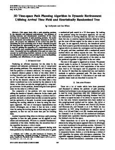
I. I NTRODUCTION Accurate sensing, obstacle detection and modeling of cluttered, unstructured scenes, such as natural outdoor environments, is a difficult research challenge. This paper develops techniques for enabling efficient three-dimensional (3-D) path planning among obstacles represented by dense point data sets. These data sets are typical of the data returned by Light Amplification for Detection and Ranging devices (LADAR). Using a priori aerial data scans of forested environments, we compute a network of free space bubbles forming safe paths within environments cluttered with tree trunks, branches and dense foliage. An example 1 of such a result is presented in Figure 1. The network of paths is used as an efficient data structure for encoding obstacle information which can be used for 3-D path planning. Recent work on real-time 3-D motion planning with moving obstacles has motivated us to look at the problem of 3-D motion planning in highly cluttered and unstructured environment. Previous work has been done in the context of computer animation and interactive graphics [3]. Here we consider planning for autonomous unmanned aerial navigation. Specifically, we explore the idea of navigation below the forest canopy for small scale, less than two meters in diameter, Unmanned Aerial Vehicles (UAV) that can maneuver in three dimensions. Such vehicles are envisioned for a variety of missions including reconnaissance. Some are small enough to be launched and recovered from an autonomous ground vehicle [11]. Several of such vehicle prototypes are under development including the Allied aerospace iSTAR and the 1 Figures

in this paper are designed to be viewed in color

0-7803-8914-X/05/$20.00 ©2005 IEEE.

Fig. 1. Illustration of the free space bubbles in a forested environment. In red, the ground surface; in green, the tree canopy; in blue, the tree trunks and finally in grey the bubbles of different diameters.

Aurora GoldenEye. Their small sizes and ducted fan make them particularly suitable for navigation in highly cluttered environments such as the tree canopy. But their low payload prevents them from carrying on-board a comprehensive sensor suite. In addition, highly cluttered terrains reduce the range of the sensor field of view, generally limiting navigation control to local reactive modes. Long range and reliable navigation requires a level of environment knowledge that cannot be produce on-board such a vehicle in such an environment. The availability and quality (density, resolution) of aerial LADAR data makes them particularly interesting as a priori information to address our problem. Such information will be provided prior to the small AUV mission by a larger UAV or a manned platform. We use data provided by the CMU Autonomous Helicopter, illustrated in Figure 4. Details on this aircraft and its mapping capabilities are presented in Section V-A. The a priori data can be used to compute three-dimensional safety tunnel networks prior to the mission. The tunnel network is stored on-board of the small UAV. In the scenario envisioned, the small UAV will track on the fly the precomputed paths but avoid local obstacle. Such approach was used successfully in 2D-1/2 for planning a priori path for a ground mobile robot during the PerceptOR program [14]. In this paper, we focus on the processing of the prior data and the tunnel network 4624

computation. This approach is designed to take advantage of the data available in our context in order to achieve navigation tasks. The use of aerial data is not advocated as a panacea for outdoor mobile robot navigation but only as one way to address some of the many challenges faced in outdoor environments. Our approach can be decomposed into two steps. First, the scene made of 3-D points is segmented into three classes (ground, vegetation, and tree trunk-branches) based on features characterizing the local 3-D geometry. Secondly, a path planning algorithm explores the segmented environment to extract connected obstacle-free areas to form a network of tunnels (network edges) intersecting at some locations (network nodes). The next section deals with 3-D data classification. Section IV gives an overview of the planning method and computation of the tunnel network. Section V contains results produced using aerial data collected with the CMU Autonomous Helicopter. II. S TATE OF THE ART The state of art we reviewed can be divided into two broad categories: 3-D path planning and UAV navigation. On one hand, several authors looked at the problem of 3D path planning using dense environment representation such as quad-tree or voxel representations [4], [8], even proposing a real-time implementation of A∗ to detect obstacle free paths in the presence of moving obstacle [7]. The geometry of the scenes considered were much simpler than the cases we propose to deal with. In the work of Brock [1] free space tunnels in the workspace are computed using a greedy wavefront expansion algorithm. We use the representational idea of tunnels of free space to search large data sets of obstacle information to compute path networks. We also build upon research in UAV navigation in natural terrain or in urban environments. Nikolos [12] proposes an off/on line planner but only for 2D-1/2 environments. Sinopoli [13] is interested in nap-of-the-earth navigation with the aircraft flying on top of the tree canopy instead of inside the canopy. Vision-based systems have also been considered for navigation in canyon-like structures such as urban environments [6], [5]. They differ from our work because the environment can be represented by simple geometric primitive (meshes and planes). Finally, Zapata [16] presented a related work which is primarily focused on reactive obstacle avoidance. III. DATA SEGMENTATION In [15], we proposed a method to classify 3-D LADAR data in natural terrain into three classes: vegetation, solid surfaces and linear structures. The method estimates the local point distribution in space and uses a Bayes classifier to produce the probability of belonging to each class. Priors are modeled as Mixtures of Gaussians and parameters are learned using the Expectation-Maximization algorithm

(EM) on labeled data. At each point, the scatter matrix is computed using a predefined support region. The principal components of this matrix are used to define three saliency features for each scale [2], characterizing the 3-D points’ spatial distribution into the three classes. We reuse here the notation introduced in [15]: if {Xi } = {(x, y, z)} is a 3-D point we wish to characterize locally, we define by B(X) = {Xk ; |Xk − X| < r} the support region with r its
extent. Xi we have: With X = N1 1  (Xi − X)(Xi − X)T covB(X) (X) = N The matrix is decomposed into principal components ordered by decreasing eigenvalues: |covB(X) (X) − λ · Id| = 0 with λ0 ≥ λ1 ≥ λ2 . The saliency features used for classification are defined as:   λ2 S =  (λ0 − λ1 ) · t  (λ1 − λ2 ) · n The direction associated with the scalar value of the saliency features, respectively the tangent (t) and the normal (n) for the linear and surface feature, is used to discriminate the tree trunks. By projecting the classified 3D points into a 2-D map and by voting on the class we can determine the center of the tree trunk. Figure 2 shows an example of terrain classification using CMU helicopter LADAR data. Note the recovery of the tree trunks and the vegetation above the ground. In Section V-A we give an overview of the mapping sensor used to produce such a data set. In addition, in Section V-B we characterize the distribution of the points for this scene. IV. P LANNING The goal of the path planner is to preprocess and convert the information from the LADAR data into a representation that could be used on-board the small UAV for navigation. A. Obstacle Distance Field First, the classified point data is used to compute a distance field on the free space. The space is discretized into cells (voxels) which will store local obstacle distance information. The minimum distance to the nearest sensed obstacle is computed and stored in each voxel, forming a distance field over the free space accurate up to the specified resolution. B. Tunnel Network The voxel centers along with their value from the distance field can be interpreted as defining a spherical ”bubble” of free space. The radius of the bubble is determined by the value in the distance field. A tunnel represents a connected sequence of overlapping bubbles between two 4625

T

τ

Connected sequence of bubbles forming a tunnel of free space of minimum width rT (i.e. all bubbles in the tunnel have a radius r ≥ rT ) Continuous path in 3 connecting qinit and qgoal lying entirely inside the tunnel T

The basic algorithm utilizes an A* search over G which is optimized for grid structures in 3 [9]. The input to the planner is the set {qinit , qgoal , G, Dmin }, where Dmin is the specified minimum required distance between the UAV and any obstacle in the environment. The cost function ρ(C1 , C2 ) →  defines an implicit metric over the set of possible solutions. The planner returns a path τ constrained to lie in an optimal tunnel T according to ρ. The minimum distance constraint is enforced to guarantee that rT ≥ Dmin . Fig. 2. Example of terrain classification. The red points represent the load bearing surface, blue points represent tree trunks and branches, and the green points correspond to foliage and other vegetation features.

points in the free space. The tunnel defines a volume of free space within which a safe path for the UAV lies. Because many such tunnels may connect any two given points, the free space is actually composed of a tunnel network, which can be stored as a graph with potentially multiple connected-components.

E. Network Construction The criteria used to determine viable tunnels between two voxel cell locations is the intersection between their corresponding bubbles of free space. Given a sphere centered at C1 with radius R1 and a sphere centered at C2 with radius R2, if the distance between their centers is greater than the sum of the radii, then the spheres are disjoint: ||C1 − C2||2 ≥ R1 + R2

C. Path Search The goal of the path search phase is to compute a continuous path connecting the initial and goal configurations of the UAV that lies safely inside the tunnel network. For the experiments in this paper, all paths consisted of a sequence of straight and diagonally-adjacent voxel cells in the grid that connects the start and goal cells while minimizing a given cost metric. Several choices for cost metrics include path length, distance to obstacles, visibility from above the canopy, or other mission criteria. D. Mathematical Formulation To formalize the problem, we define the following terms: G qinit Cinit qgoal Cgoal ρ(C) P Bijk

3D occupancy grid of the environment Initial configuration of the UAV Cell in G corresponding to qinit Goal configuration of the UAV Cell in G corresponding to qgoal Metric cost function used to evaluate a voxel cell C An ordered sequence of cells in G connecting Cinit and Cgoal Spherical “bubble” of free space of radius rijk centered at voxel cell Cijk

R2

x R1 C2

R2

R1

C1

C1

C2

d

Fig. 3. Left: Calculating the size of the connecting hole between two overlapping spheres. Right: Interior spheres (spheres lying wholly within a larger sphere) are pruned from the tunnel network.

If their volumes intersect, then we first test whether either of the spheres is entirely contained within the other as in Figure 3 (right). This condition is true when either: ||C1 − C2||2 + R1 < R2 or ||C1 − C2||2 + R2 < R1 holds. Otherwise, we calculate the radius of the circular hole connecting the two spherical volumes as shown in Figure 3 (left). The radius of the hole is given by: 1 2 2 4d R1 − (d2 − R12 − R22 )2 x= 2d 4626

V. R ESULTS In this section we present the aerial mapping helicopter used to collect the aerial data presented in this paper. Note that this platform is not the one considered to navigate through the canopy. We give also details on the point distribution in the environment we experimented in. We then present and analyze results of path in the canopy. Finally we look at the computational performances of our approach. A. Aerial data The CMU autonomous helicopter, illustrated Figure 4, is a versatile platform build around the Yamaha R-Max helicopter and equipped with on-board sensing which includes an IMU (LN-200 Litton), CCD Cameras (Sony 1Kx1K), GPS (Carrier phase dual freq type), a laser scanner (built around Riegl LD90-3 and that includes a registered color sensor), re-configurable on-board computing (TI DSP, Intel P3, etc), a modular sensor mount for experimental sensor deployment, power, communication, and a control system. Terrain mapping has been performed extensively over various nature of terrain (urban, natural with vegetation, desert canyons). The modified Riegl laser range finder is capable of collecting 3-D color data, with 10 cm accuracy [10].

points. For each 3-D point, the position and the attitude of the helicopter is known. Figure 9 shows a top view of the scene with the elevation color coded. The data were collected in the Fall season. B. Tree canopy voids Before extracting 3-D safety tunnels we would like to quantify the voids in the tree canopy. We consider here a global and a local measure: the occupancy rate of the space and the distribution of the diameter of free space bubbles. The data are sparsely distributed in 3-D as shown in Table I. For different voxel sizes, the occupancy rate is computed. This is a global characterization. A characterization, more relevant to our application, that preserves information about the local scene structure, is the estimation of the distribution of the free space bubbles inside the canopy. Figure 7 illustrates the cumulative distribution of the free space bubble radius. This graph shows us that 80% of the free space inside tree canopy is at least 50 cm away from obstacle. So for the 72 cm diameter iSTAR or the 1.7 m diameter GoldenEye, respectively 60 and 20 percent of the free space is accessible to them, in our example. Figure 6 shows the free space bubbles, 2 meters in diameter at least, in the scene. We can see that they merge together to form tunnels. TABLE I 3-D SPACE OCCUPANCY Grid size (m) 0.5 1.0 2.0

Fig. 4.

Empty cells 13,610,910 1,654,917 189,835

Occupied cells 367,286 119,955 32,771

Occupancy rate 2.6 6.7 14.7

Aerial mapping platform: CMU Autonomous Helicopter.

For comparison, we show in Figure 5 a ducted fan UAV considered for going through the canopy [11]. The illustration depicts the work perform in the Autonomous UAV Mission System (AUMS) project. This is a 29 inches diameter version, smaller versions exist.

(a)

(b)

Fig. 6. Illustration of the free space bubbles for the example presented in Figure 1. Only one meter radius bubbles are represented. (a) Top view. (b) Side view.

C. Paths through the canopy

Fig. 5.

Example of ducted fan UAV [11].

The data set used covers an area of 165×296×35 m and is made of more than seven millions 3-D LADAR data

To improve the visibility of the results, we present paths generated on a small section of the full data set. We choose this section of the terrain because of the height density of the tree canopy but also because of the presence of understory vegetation (bushes). Figure 8 shows : (a) the shortest but with minimum bubble radius guarantee of one meter and the safest path, (b) the safest path overlaid in 4627

Sphere radius cumulative distribution 100

percentage

80

60

40

20

0

0

2

4 radius (m)

6

8

Fig. 7. Cumulative distribution of the free space bubble radius for the cropped data set

the classified data, (c) a different view point of (b). We choose a start and a goal point at the edge of the map, well above the ground. The path produced is as expected. A robot following this path would have to lower its altitude to avoid the lower part the tree canopy, closing to the ground, then it will have increase this elevation to avoid the bushes covering the ground. Tree trucks are also avoided. Notice the size variation of the bubbles. In this example, we constrained the path to be inside the canopy, prohibiting overfly of it. D. Complete data set In this section we present results produced using the complete data set. Figure 9 shows the shortest path computed within the tree canopy. Figure 10 details the result. In Figure 10-(a) the safest and shortest path are represented. In that case we did not constrained the path so the the upper path is above the canopy while the lower path is within the canopy as illustrated in Figure 10-(b)-(c). E. Planning Performance We conducted experiments using several LADAR data sets of unstructured natural environments. The computational performance depends on the size and resolution (discretization) of the data set, as well as the cutoff minimum distances used to calculate the tunnel network. Some results are shown in Table II. All performance data was calculated using a standard PC with 1 GB of RAM and a 1.6 GHz Pentium M processor, and the reported times include the time to load the data set from disk. Times are reported for calculating a single path in the environment and for computing the entire tunnel network.

Fig. 9. Full data set used for planning. The scene is color coded based on the elevation, red being high elevation data. The grey spheres are the bubbles of free space producing the shortest path. TABLE II P LANNING P ERFORMANCE FOR THE FULL DATA SET.

Environment Data set Cropped Forest(5.0 m) Forest(2.5 m) Forest(1.0 m)

Grid size (resolution) 31x31x24 34x60x8 67x119x15 166x297x36

Free cells (voxels) 5,545 12,133 98,933 1,654,917

Time (sec.) Single Path Network 0.6 3.4 0.8 2.8 2.1 8.2 20.5 133.5

VI. C ONCLUSIONS In this paper we presented an approach for small scale UAV navigation within and below the tree canopy using a priori aerial LADAR data. 3-D safety tunnels are constructed by exploring segmented data. We demonstrated

our approach using aerial data collected by the CMU Autonomous helicopter. Other applications can be envisioned. For example by constraining the free space bubbles to intersect the ground we can find safety tunnel for ground 4628

(a)

(b)

(c)

Fig. 8. Path planning example: (a) Shortest (red) and safest (blue) paths. (b)-(c) Safest path overlayed on top of the terrain classification results: the path (grey), the ground surface (red), the vegetation (green), and linear structures such as trunks and branches (red)

(a)

(b)

(c)

Fig. 10. Details on the experiments with the full data data set: (a) Shortest (bottom) and safest (top) path, (b) Close view of the entry point into the canopy, (c) Path inside the canopy. For (b)-(c) the path is in grey, the point cloud is color coded based on the elevation.

vehicles. Also the tree canopy structure is important to model chemistry exchange, illuminations in environmental science. Future work will include comparison with ground based vehicle laser data, comparison between paths computed with data collected at different seasons. ACKNOWLEDGMENT This work is partially supported by NSF grants ECS0325383, ECS-0326095, and ANI-0224419. R EFERENCES [1] O. Brock and L. Kavraki. Decomposition-based motion planning: A framework for real-time motion planning in high-dimensional configuration spaces. In IEEE International Conference on Robotics and Automation, 2001. [2] Chi-Keung Tang Gerard G. Medioni, Mi-Suen Lee. A Computational Framework for Segmentation and Grouping. Elsevier, 2000. [3] J. Go, T. Vuand, and J. Kuffner. Autonomous behaviors for interactive vehicle animations. In Eurographics/ACMSIGGRAH Symposium on Computer Animation, 2004. [4] M. Herman. Fast, three-dimensional, collision-free motion planning. In IEEE International Conference on Robotics and Automation, 1986. [5] S. Hrabar and G. Sukhatme. Omnidirectional vision for an autonomous helicopter. In IEEE International Conference on Robotics and Automation, 2003. [6] S. Hrabar and G. Sukhatme. A comparison of two camera configurations for optic-flow based navigation of a uav through urban canyons. In EEE/RSJ International Conference on Intelligent Robots and Systems, 2004.

[7] Y. Kitamura, T. Tanaka, F. Kishino, and M.Yachida. Real-time path planning in a dynamic 3-d environment. In IEEE/RSJ International Conference on Intelligent Robots and Systems, 1996. [8] Y. Kitamura, T. Tanaka, F. Kishino, and M. Yachida. 3-d path planning in a dynamic environment using an octree and an artificial potential field. In IEEE/RSJ International Conference on Intelligent Robots and Systems, 1995. [9] J.J. Kuffner. Efficient optimal search of euclidean-cost grids and lattices. In IEEE/RSJ Int. Conf. on Intelligent Robots and Systems (IROS’04), 2004. [10] J. R. Miller. 3-D Color Terrain Modeling System for Small Autonomous Helicopters. PhD thesis, arnegie Mellon University, 2002. [11] K. Mullens and al. An automated uav mission system. In AUVSI Unmanned Systems in International Security, 2003. [12] I. Nikolos, K. Valavanis, N. Tsourveloudis, and A. Kostaras. Evolutionary algorithm based offline/online path planner for uav navigation. In IEEE Transactions on Systems, Man and Cybernetics, 2003. [13] B. Sinopoli, M. Micheli, G. Donata, and T. Koo. Vision based navigation for an unmanned aerial vehicle. In IEEE International Conference on Robotics and Automation, 2001. [14] N. Vandapel, R. Donamukkala, and M. Hebert. Experimental results in using aerial ladar data for mobile robot navigation. In International Conference on Field and Service Robotics, 2003. [15] N. Vandapel, D. F. Huber, A. Kapuria, and M. Hebert. Natural terrain classification using 3-d ladar data. In IEEE International Conference on Robotics and Automation, 2004. [16] R. Zapata and P. Lepinay. Flying amoong obstacles. In European Workshop on Advanced Mobile Robots, 1999.

4629