D47 (1993) 5128. 9] S. G. G usken, Nucl. Phys. B (Proc. Suppl.) 17 (1990) 361; C. Alexandrou, S. G. G usken,. F. Jegerlehner, K. Schilling and R. Sommer, Nucl.
DESY 95-128 HLRZ 95-36 HUB-EP-95/9 June 1995
Polarized and Unpolarized Nucleon Structure Functions from Lattice QCD M. Gockeler , R. Horsley , E.-M. Ilgenfritz , H. Perlt , P. Rakow , G. Schierholz and A. Schiller 1;2
1;3
3
6;1
hep-lat/9508004 11 Sep 1995
1
4
5
4
Hochstleistungsrechenzentrum HLRZ, c/o Forschungszentrum Julich, D-52425 Julich, Germany Institut fur Theoretische Physik, RWTH Aachen, D-52056 Aachen, Germany Institut fur Physik, Humboldt-Universitat, D-10115 Berlin, Germany Fakultat fur Physik und Geowissenschaften, Universitat Leipzig, D-04109 Leipzig, Germany Institut fur Theoretische Physik, Freie Universitat, D-14195 Berlin, Germany Deutsches Elektronen-Synchrotron DESY, D-22603 Hamburg, Germany 2
3
4
5
6
Abstract
We report on a high statistics quenched lattice QCD calculation of the deep-inelastic structure functions F1, F2 , g1 and g2 of the proton and neutron. The theoretical basis for the calculation is the operator product expansion. We consider the moments of the leading twist operators up to spin four. Using Wilson fermions the calculation is done for three values of �, and we perform the extrapolation to the chiral limit. The renormalization constants, which lead us from lattice to continuum operators, are calculated in perturbation theory to one loop order.
1
1 Introduction Deep-inelastic lepton-nucleon scattering is described by four structure functions: F1, F2, g1 and g2. The spin-averaged structure functions F1 and F2 carry information about the overall density of quarks and gluons in the nucleon. They have played a seminal role in the development of our current understanding of the structure of hadrons. The polarized structure function g1 goes one step further and probes the distribution of quarks of a given helicity in the longitudinally polarized nucleon. Recent measurements of g1 [1] have revealed the (at rst sight) surprising result that only a small fraction of the nucleon's spin is carried by quarks. This has triggered a great deal of interest in the subject. The other polarized structure function g2 has no interpretation in purely partonic language. It involves a twistthree operator and thus o�ers the rst direct measurement of higher twist operator matrix elements [2]. Experiments that measure g2 are currently being performed at DESY and SLAC. We have initiated a program to compute F1, F2, g1 and g2 on the lattice [3]. For an earlier attempt to compute the unpolarized structure functions see [4]. The theoretical basis for such a calculation is the operator product expansion (OPE), which relates the moments of the structure functions to forward nucleon matrix elements of certain local operators. Where a parton model interpretation exists, it can be mapped onto an OPE analysis. Our calculation will be in the quenched approximation, where internal quark loops are neglected. In this paper we shall also neglect gluonic operators, which contribute only to higher order in the coupling constant expansion. For the unpolarized structure functions we then have for the leading twist contribution 2
Z
1
0
Z
1 0
dxxn 1F1(x; Q2) = dxxn 2F2(x; Q2) =
X (f ) 2 2 c1;n(� =Q ; g(�)) vn(f )(�);
f =u;d
X (f ) 2 2 c2;n(� =Q ; g(�)) vn(f )(�)
f =u;d
(1)
for n � 2 (generally even n), where 1 Xh~p;~sjO(f ) j~p;~si = 2v(f )[p � � � p traces]; � n �1 f�1���� g 2 ~s � i �n 1 $ ( f ) � �1 $ traces (2) D �2 � � � D � O�1���� = 2 with = u(d) for f = u(d), and c(1f;n)(�2=Q2; g(�)) = Q(f )2(1 + g(�)2c�1;n(�2=Q2; g(�))); c(2f;n)(�2=Q2; g(�)) = Q(f )2(1 + g(�)2c�2;n(�2=Q2; g(�))): (3) Here � denotes the subtraction point, and f� � �g indicates symmetrization. We have chosen the normalization h~p;~sj~p 0;~s 0i = (2�)32E~p �(~p ~p 0)�~s;~s ; s2 = m2N . The moments of F1, F2 have the parton model interpretation (4) vn(f ) = hxn 1i(f ); n
n
n
n
0
2
where x is the fraction of the nucleon momentum carried by the quarks. In the quenched approximation the above-mentioned equations hold for odd n as well. For the polarized structure functions we have, again for the leading twist contribution, Z1 X (f ) 2 2 2 0 dxxng1(x; Q2) = 21 e1;n(� =Q ; g(�)) a(nf )(�); (5) f =u;d Z1 n X [e(f )(�2=Q2; g(�)) d(f )(�) e(f )(�2=Q2; g(�)) a(f )(�)] (6) 2 dxxng2(x; Q2) = 12 n + 1;n n n 1 f =u;d 2;n 0 for even n and n � 0 (n � 2) for g1 (g2), where [2] h~p;~sjOf5(��f )1���� gj~p;~si = n +1 1 a(nf )[s� p�1 � � � p� + � � � traces]; h~p;~sjO[5(�ff�)1]���� gj~p;~si = n +1 1 d(nf )[(s�p�1 s�1 p� )p�2 � � � p� + � � � traces]; � i �n $ 5( f ) D �1 � � � D � traces O��1 ���� = 2 � � 5$ and e(1f;n)(�2=Q2; g(�)) = Q(f )2(1 + g(�)2e�1;n(�2=Q2; g(�))); e(2f;n)(�2=Q2; g(�)) = Q(f )2(1 + g(�)2e�2;n(�2=Q2; g(�))): In eq. (7) [� � �] indicates antisymmetrization. In parton model language n
n
n
n
(7)
n
n
(8)
a(0u) = 2�u; a(0d) = 2�d; (9) where �u; �d determine the fraction of the nucleon spin that is carried by the quarks. A similar interpretation holds for the higher spin operators. The structure function g2 consists of two contributions: a(nf ) is the so-called Wandzura-Wilczek contribution [5] which corresponds to twist two, whereas d(nf ) corresponds to twist three. In addition to d(nf ) there is a contribution to g2 from a twist-three operator which is proportional to the quark mass [6]. Since we are mainly interested in the chiral limit we have neglected that.
2 Lattice Calculation
We perform our quenched QCD calculations for Wilson fermions with r = 1 on a 163 � 32 lattice. For the gauge coupling we take � 6=g2 = 6.0. To be able to extrapolate our results to the chiral limit, we run at three di�erent hopping parameters, � = 0:155; 0:153 and 0:1515. This corresponds to physical quark masses mq of roughly 70, 130 and 190 MeV, respectively, using the perturbative relation (10) mqa = 0:56( �1 �1 ); c where a is the lattice spacing. 3
For the gauge update we use a cycle consisting of a single three-hit Metropolis sweep followed by 16 overrelaxation sweeps [7]. We repeat this cycle 50 times in order to generate a new con guration. The resulting con gurations seem to be independent. We see no correlations between hadronic quantities calculated on di�erent gauge eld con gurations. The calculations are carried out on Quadrics Q16 and QH2 parallel computers. For details of the implementation of our code on these machines see [3]. So far we have collected of the order 1000, 600 and 400 independent con gurations at the three � values. To calculate the nucleon matrix elements we rst compute two- and three-point correlation functions de ned by X C (t; ~p) = ;� hB� (t; ~p)B� (0; ~p)i;
C (t; �; p~; O) =
�;
X �;
;� hB� (t; ~p)O(� )B� (0; p~)i:
(11)
The lattice operators O used here are obtained from the operators in the euclidean continuum, which look exactly like the operators in eqs. (2), (7) up to ! factors of i, by replacing the covariant derivative by the lattice covariant derivative so that D � becomes ! D �(x; y) = 12 [U�(x)�y;x+^� U�y (x �^)�y;x �^]: (12) We write the ratio of three- to two-point correlation functions as R(t; �; p~; ; O) = C (t; �;~p; O)=C 12 (1+ 4)(t; p~) E~p F ( ; J ) (13) = 21� E + ~p mN (for 0 � � � t) with F ( ; J ) = 41 Tr [ N J N ] ; N = 4 i~p~ =E~p + mN =E~p (14) and J de ned by h~p;~sjOj~p;~si = u�(~p;~s)J u(~p;~s): (15) When calculating three-point functions it is particularly important that the baryon operator B has only little overlap with excited baryon states, in order to make the plateau region in � as broad as possible. As our basic proton operator we use (with C = 4 2 in our representation) X i~p~x B�(t; ~p) = e �abcua�(x)(ub(x)C 5dc(x)) (16) ~x;a;b;c
with two important improvements. First we use `Jacobi smearing' [8] (a version of [9]) in order to have an extended proton operator. Thus each quark operator in eq. (11) is replaced by N X D )n ; (17) ! S = (�s ! s
n=0
4
E
eff N
m
p=2π /16
2 N
t
eff
m
N
2 mρ
2 mπ
p=0
1/ κ
t (a)
(b)
Figure 1: (a) E�ective nucleon mass plot for ~p = 0 (bottom), and e�ective nucleon energy plot for j~pj = 2�=16 (top) at � = 0:155. Both source and sink are smeared. The horizontal lines indicate the result of the t as well as the t interval. (b) m2� , m2� and m2N as a function of 1=� together with other recent results of the literature: this work, 2 Ref. [10], 3 Ref. [11], 4 Ref. [12]. The t to all data points combined gives �c = 0:15699(5).
5
m� m� mN
� 0.1515 0.153 0.504(2) 0.422(2) 0.570(2) 0.507(2) 0.900(5) 0.798(5)
0.155 0.297(2) 0.422(2) 0.658(5)
Table 1: The hadron masses in lattice units at = 6:0. and similarly for � as we smear both source and sink. We found suitable values of the parameters to be Ns = 50; �s = 0:21, which for our largest � value gave a rms radius of about 4, corresponding roughly to 0.5 fm, i.e. half the nucleon radius. Secondly we replace each spinor by (18) ! NR = 21 (1 + 4) ; � ! �NR = � 12 (1 + 4): This replacement leaves quantum numbers unchanged, but we expect it to improve overlap with those baryons which have slow-moving valence quarks. Practically this means that for each baryon propagator we invert on a smeared local source and consider only the rst two Dirac components. So we only have 2 � 3 inversions to perform rather than the usual 4 � 3 inversions, which saves a factor two in computer time in the inversion. In Ref. [3] we have seen that the projection (18) is particularly e�ective at reducing unwanted backward propagating states, which extends the window that one can practically use for matrix element calculations to well above half the temporal extent of the lattice. In Fig. 1a we show a plot of the resulting e�ective nucleon energy, as given by ln(C (t)=C (t +1)), for ~p = 0 and j~pj = 2�=16 at our smallest quark mass. For zero nucleon momentum we nd a good plateau with a proton mass of 0.658(5). For the lowest non-zero momentum we nd an energy of 0.765(11), which is in good agreement with the continuum dispersion relation. In both cases we see that after a distance of about four time units there is very little trace of an excited state. In Table 1 we give the mass values of the nucleon together with those of the � and � for our three values of �. The chiral limit is obtained by extrapolating in 1=� to zero � mass. Assuming, as usual, that m2� depends linearly on 1=�, we obtain from our data the critical value �c = 0:15693(4). In Fig. 1b we plot m2� , m2� and m2N as a function of 1=�. In this plot we have also included other recent results at = 6:0. A combined t gives mN =m� = 1:37 in the chiral limit. To calculate three-point functions we require additional propagators, one for each chosen t, p~ and . We have xed t at 13 and have chosen = 21 (1 + 4), corresponding to the unpolarized case, and = 21 (1 + 4)i 5 2, corresponding to polarization (+ - ) in the 2direction. For the momentum we have taken ~p = 0 and ~p = (2�=16; 0; 0) � (p1 ; 0; 0). We have also considered = u, d separately. This means that we must nd 2 � 2 � 2 = 8 (half) quark propagators. The choice t = 13 is su�cient. Larger values of t lead to unacceptably large errors in the signal for R. Test runs for t = 17 turned out to have O(2) larger errors, which roughly corresponds to the increase in the noise in the baryon correlation function from t = 13 to t = 17. 6
hOi
Components
v2;a Of14g v2;b Of44g 13 (Of11g + Of22g + Of33g) v3 Of114g 12 (Of224g + Of334g) v4 Of1144g + Of2233g Of1133g Of2244g a0 O25 a2 Of5214g d2 O[25 f1]4g
Representation Ref. [13] Ref. [14] �3(6) 6(+) (+) �1(3) �1(8) 8(+) (+) �1(2) �4(4) ( 12 ; 21 )( ) �3(4) ( 12 ; 21 )(+) �1(8) 8(+)
C + + + + + +
Table 2: The lattice operators and their representation. The momentum is taken to be p~ = (2�=16; 0; 0) � (p1; 0; 0) in the case of v2;a; v3; v4; a2; d2 and ~p = 0 elsewhere. C denotes charge conjugation.
3 Lattice Operators and their Renormalization
The bare lattice operators, O(a), are in general divergent. We de ne nite operators O(�), renormalized at the scale �, by O(�) = ZO ((a�)2; g(a))O(a); (19) where
(20) hq(p)jO(�)jq(p)i = hq(p)jO(a)jq(p)i jtree p =� with jq(p)i being a quark state of momentum p. In the limit a ! 0 this de nition amounts 2
2
to the continuum, momentum subtraction renormalization scheme. The lattice operators transform under the discrete hypercubic group H (4) [13, 14]. They must be constructed such that they belong to a de nite irreducible representation of the latter. In particular they must not mix with lower-dimensional operators. This is prerequisite to the operators being multiplicatively renormalizable. Furthermore, from the more practical point of view, the operators should only require a non-zero spatial momentum in at most one direction. We have considered the operators listed in Table 2. For the group theoretical classi cation of the lattice operators see Ref. [15]. The calculation of v2;a, v3, v4, a2 and d2 requires non-vanishing nucleon momenta. Note that for the quenched theory there is no mixing with gluon operators. In the continuum limit the matrix elements v2;a and v2;b should be equal. At nite lattice spacing this provides us with a consistency check and gives information about possible lattice artifacts. We have computed the renormalization constants for our operators in the quenched approximation for Wilson fermions in perturbation theory to one loop order. For this task 7
hOi v2;a v2;b v3 v4 a0 a2 d2
O
BO ZO (1; g = 1:0) 16 -3.165(6) 1.0267(1) 3 16 -1.892(6) 1.0160(1) 3 25 fgfg: 3 -19.572(10) 1.1653(1) fg(): 0 0.370(10) -0.0031(1) 157 -37.16(30) 1.314(3) 15 0 15.795(3) 0.8666(0) 25 -19.560(10) 1.1652(1) 3 7 -15.680(10) 1.1324(1) 3
BOMS - 409 - 409 - 679 - 2216 225 0 - 679 - 13 12
Table 3: The renormalization constants in the quenched approximation. The errors quoted are a conservative estimate of the uncertainties in the numerical evaluation of the integrals involved. The numbers in the rightmost column represent the contribution of the continuum operators computed in the MS scheme. we have developed packages of computer algebraic programs using Mathematica and Maple to such a level that all what is needed as input is to state the Feynman rules in symbolic form, both for the continuum and the lattice part of the calculation. We will summarize our results here. A detailed account of our calculation will be given elsewhere [16]. In the case of v3 it turns out that the operator Of114g 21 (Of224g + Of334g) mixes with the operator [15] (21) O(114) 12 (O(224) + O(334)); O(���) = O��� + O��� 2O��� under renormalization. This operator is of mixed symmetry, is traceless and corresponds to the representation 8(+); C = as well. Thus we have
Ofg(�) = ZfgfgOfg(a) + Zfg()O()(a);
(22)
where we have used a short-hand notation for the operators in Table 2 and eq. (21). We write (CF = 4=3) 2 (23) ZO ((a�)2; g) = 11 16g�2 CF [ O ln(a�) + BO ]: This is to be interpreted as a matrix equation in the case of v3. Our results for the anomalous dimensions O and the BO 's are given in Table 3 for r = 1. The renormalization constants Zv2 and Za0 have been given before in the literature [17, 18, 19]. We agree with the results of these authors. In the case of v3 the o�-diagonal component of Z is negligibly small. ;b
8
The structure functions do not depend on �, but hxn 1 i and �u, �d do. In the following we shall quote our results for �2 = Q2 = a 2 � 2GeV2; (24) which eliminates the logarithms in the Wilson coe�cients and renormalization constants, and we will denote ZO (1; g = 1:0) by ZO . The corresponding numerical values are also listed in Table 3. As the Wilson coe�cients are generally computed in the MS regularization scheme, one needs to know the renormalization constants in this scheme too. In Table 3 we state the contribution of the continuum operators computed in the MS scheme. The di�erence of the BO 's then gives the result in the MS scheme. The renormalization constants receive contributions from ve di�erent types of diagrams: the vertex, the leg self-energy, the leg tadpole, the operator tadpole and the operator comb diagrams. The tadpole diagrams give by far the largest contribution to the renormalization constants. The leg tadpole contribution is the same for all operators. The operator tadpole contribution is proportional to the number of covariant derivatives and has opposite sign to the leg tadpole. Leg and operator tadpole diagrams cancel each other in v2. This accounts for the small values of Bv2 ; Bv2 . In a0 only the leg tadpole contributes. In all other cases it is the operator tadpole diagram which dominates. ;a
;b
4 Structure Function Results The next step is to calculate the ratio of three- to two-point correlation functions R, as given in eq. (13), for the operators listed in Table 2. To make sure that we are computing the matrix elements of the lowest-lying state, i.e. the nucleon, we must look for plateaus in � , the time distance of the operator from the source, for 0 � � � t = 13. In Fig. 2 we show R as a function of � for six of our operators at � = 0:153. The ratio Rv2 not shown here is of the same quality as Rv2 . We nd in all cases that the signal is practically constant for time distances larger than two lattice spacings from the source and from the sink. For 13 � � the signal is practically zero as one would expect. The t interval is taken to be 4 � � � 9. The result of the t is shown by the horizontal lines, and the errors are indicated by the dotted lines. The renormalized operator matrix elements are obtained from the ratio R by Rv2 = Z i 21� p1v2;a; Rv2 = Z1 21� mN v2;b; v2 v2 Rv4 = Z1 21� Ep1 p21 v4; Rv3 = Z1 21� p21 v3; v3 v4 (25) i 1 1 m 1 1 N Ra0 = Z 2� 2E a0; Ra2 = Z 2� 6 mN p1a2; a0 p1 a2 Rd2 = Z1 21� 31 mN p1 d2: d2 ;b
;a
;a
;b
;a
;b
9
u
u
d
d d
u
(a)
(c)
(b)
u u
d d
u d
(d)
(e)
(f)
Figure 2: The ratio R for u and d quark insertions for � = 0:153. (a) -iRv2 , (b) Rv3 , (c) Rv4 , (d) -iRa0 , (e) Ra2 and (f) Rd2 . Both source and sink are smeared. The source is at t = 0, the sink at t = 13. ;a
10
p
We have de ned the continuum quark elds by 2� times the lattice quark elds. For the renormalization constants we take the perturbative values given in Table 3 and Zv4 = 1. In the case of v3 we have also computed the nucleon matrix element of the operator in eq. (21). It turned out to be noisy and consistent with zero within an error of roughly 1/5 the magnitude of the leading symmetric contribution. Given the small o�-diagonal component of the renormalization constant, we may thus safely neglect the e�ect of mixing. Tadpole resummation [20] would leave Zv2 , Zv2 unchanged, while it would change the other renormalization constants by a few percent. The exact amount depends on how it is implemented, and there is considerable freedom to do so. (Better is to compute the renormalization constants non-perturbatively [21] what we are doing now [22].) The results are plotted in Fig. 3, and the numerical values are listed in Table 4. All our results are given for the proton. The distribution functions of the neutron are obtained by interchanging u and d. We shall now discuss our results in detail. The rst important observation to make is that the values of hxia and hxib, which are obtained from di�erent representations of the hypercubic group H (4) (cf. Table 2), are consistent with each other, within the error bars. This indicates that lattice artifacts are presumably small. A second observation is that all matrix elements show roughly a linear behavior in 1=�, i.e. in the quark mass (cf. eq. (10)). The lines shown in Fig. 3 are linear ts to the data. The result of the extrapolation is indicated by the solid circles and the solid box, and the numerical values of the t are given in the last column of Table 4. Let us concentrate on the moments of the unpolarized structure functions rst. We see that the lowest moment (n = 2) is practically independent of the quark mass. For growing n the moments show a stronger and stronger increase with the quark mass. For the distribution function itself this means that at small x quark mass e�ects are negligible, while at intermediate and large x its shape depends strongly on the magnitude of the quark mass. In the limit of large quark masses the higher moments approach the predictions of the nonrelativistic quark model. In particular we nd hxn 1 i(u) � 2hxn 1 i(d) for all n. In the chiral limit the picture changes completely. Whereas at small x the ratio of u to d distribution is roughly two, the ratio increases rapidly for larger values of x. We may compare our results in the chiral limit with the phenomenological valence quark distribution functions. In Fig. 3a-c we show the results of a recent such t [23]. For n = 2 the lattice values are signi cantly larger than the phenomenological values, for n = 3 they are about equal within the statistical errors, and for n = 4 the lattice values are signi cantly smaller than the phenomenological values. This holds for both, u and d quark distributions. Thus, our calculation predicts a valence quark distribution function that is more singular at small x than the phenomenological one, i.e. has a somewhat larger Regge intercept. At the moment we have no explanation for this discrepancy. According to our calculation 64% of the nucleon's momentum is carried by the (valence) quarks. We shall now turn to the discussion of the polarized structure functions. Let us rst focus on �u and �d, which in the quenched approximation determine the fraction of the proton spin that is carried by the valence quarks. Sea quark e�ects may be neglected for ;a
11
;b
u u u
d d
d
(a)
(b)
(c)
u u
d
d
u d
(d)
(e)
(f)
Figure 3: The moments of the proton structure functions as a function of 1=�, together with a linear t to the data. The solid symbols indicate the extrapolation to the chiral limit. In (a) circles refer to hxia, boxes to hxib . In (a-c) we compare our results with the phenomenological valence quark distribution of Ref. [23] ( t D ). The phenomenological moments are marked by asterisks. In (d) we compare our numbers with the phenomenological values of Ref. [24], which are marked by asterisks as well. (The value for �u is hidden behind the lattice number.) 12
Observable
hxia hxi(bu) hxi(av:u) hxi(ad) hxi(bd) hxi(av:d) hx2i(u) hx2i(d) hx3i(u) hx3i(d) (u)
�u �d a(2u) a(2d) d(2u) d(2d)
0.1515 0.477(23) 0.478(22) 0.478(16) 0.226(11) 0.226(10) 0.226(08) 0.147(11) 0.066(05) 0.060(05) 0.026(03) 0.938(45) -0.250(12) 0.170(10) -0.037(03) -0.110(05) 0.020(02)
0.153 0.436(20) 0.473(20) 0.455(14) 0.201(10) 0.219(09) 0.210(07) 0.127(10) 0.056(05) 0.049(05) 0.018(03) 0.935(44) -0.250(12) 0.165(11) -0.037(04) -0.138(07) 0.024(02)
�
0.155 �c = 0:1569 0.457(28) 0.430(43) 0.475(20) 0.473(32) 0.466(16) 0.452(26) 0.195(12) 0.174(20) 0.211(09) 0.204(15) 0.203(07) 0.189(12) 0.122(13) 0.104(20) 0.047(06) 0.037(10) 0.035(08) 0.022(11) 0.008(04) -0.001(07) 0.863(43) 0.830(70) -0.246(14) -0.244(22) 0.161(20) 0.154(27) -0.051(10) -0.050(12) -0.201(16) -0.233(20) 0.036(06) 0.040(07)
Table 4: Structure function results for the proton. All numbers refer to the momentum subtraction scheme. heavy quarks, and they drop out in the di�erence �u �d. In the chiral limit we obtain �u �d � gA = 1:07(9): (26) This is to be compared with the experimental value of the axial vector coupling constant gA = 1:26. In Fig. 3d we compare �u and �d individually with a recent phenomenological t of the polarized structure function data [24], which naturally includes sea quark e�ects. If we add the sea quark contribution to our results { a recent lattice calculation [25] nds ��u = �d� = 0:14(5), ��s = 0:13(4) using perturbative renormalization factors { we would favor a somewhat smaller value for �u than the tted value. For the total quark spin contribution to the nucleon spin we would furthermore obtain �� = 0:18(8), in agreement with the result of a full QCD calculation [26], i.e. including dynamical quarks. For heavy quark masses we nd �u � 1 and �d � 1=4, in good agreement with the three-quark model [27]. By comparing the moments a0 = 2�q and a2 with those of the unpolarized structure functions we nd that in the chiral limit g1 is less singular than F1 as x goes to zero. This is also what one nds experimentally [28]. In the limit of large quark masses, on the other hand, it seems that g1 is proportional to F1. 13
If we combine our results with the perturbatively known [29] Wilson coe�cients we can compute the moments of g1. In the chiral limit we obtain for the lowest moment Z1 0
dxg1(x; Q = 2)
(
0:166(16) proton; 0:008(09) neutron:
(27)
Remember that Q2 � 2GeV2. For the di�erence of proton and neutron structure functions we nd Z1 dx(g1p(x; Q2) g1n (x; Q2)) = 0:174(15): (28) 0 This is the quantity which should be compared with experiment, because here the sea quark contribution drops out. Our result is in good agreement with the phenomenological analysis [24, 28]. In the higher moments of g1 sea quark e�ects should not play any role anymore either. In the chiral limit we obtain ( Z1 proton; 2 2 dxx g1(x; Q ) = 00::0150(32) (29) 0012(20) neutron: 0 Here we have converted the renormalization constants to the MS scheme, because the Wilson coe�cients were computed in this scheme too. This result is consistent with experiment [30]. Let us nally discuss the structure function g2. From Fig. 3f we read o� that the twistthree contribution d2 is strongly mass dependent. While d2 approaches zero in the heavy quark limit, for both u and d quark insertion, it is of the same order of magnitude as its twist-two counterpart a2 for small quark masses. In the chiral limit we obtain Z1 0
dxx g2(x; Q = 2
2)
(
0:0161(16) 0:0100(22) = 0:0013(09) + 0:0009(13) =
0:0261(38) proton; 0:0004(22) neutron:
(30)
As before, Wilson coe�cents [29] and renormalization constants are consistently computed in the MS scheme. In eq. (30) the rst number comes from d2, while the second number comes from a2 (cf. eq. (6)). We see that the twist-three operator provides the dominant contribution. The Wandzura-Wilczek description of g2 [5] is a valid approximation for large quark masses, but for light quark masses it is de nitely not. Our results seem to be in disagreement with recent estimates based on sum rules [31], which suggest that for the proton d2 is very small.
5 Conclusion We have presented results of a calculation of the lower moments of the polarized and unpolarized deep-inelastic structure functions of the nucleon. The calculation has been performed in the quenched approximation, where sea quark e�ects are neglected, and it was done for three di�erent quark masses. This allowed us to extrapolate our results to the chiral limit. The valence quark distributions that we have obtained di�er somewhat from the phenomenological ones [23]. One explanation could be that at smaller values of Q2 higher twist 14
contributions are non-negligible, which have not been included in the phenomenological analysis. We plan to investigate this possibility in the future. Our results for the polarized structure functions are consistent with experiment, as far as data exist. A surprise was that the twist-three operator contributed so much to g2. It was interesting to see how the results varied with the quark mass. At large quark masses our results agree largely with what one would expect on the basis of the quark model. For small quark masses there are, however, signi cant changes. With the (raw) lattice data being relatively accurate now, the calculation of the renormalization constants has become a major issue. So far we have computed the renormalization constants in perturbation theory to one loop order. We hope to do better in the near future [22]. The renormalization constant for v3 has independently been computed by the Rome group [32]. We have compared our results with theirs at intermediate stages of the calculation, and they agreed. These authors use a slightly di�erent basis of operators from ours though.
Acknowledgments This work was supported in part by the Deutsche Forschungsgemeinschaft. The numerical calculations were performed on the Quadrics parallel computers at Bielefeld University and at DESY (Zeuthen). We wish to thank both institutions for their support and in particular the system managers M. Plagge and H. Simma for their help. We furthermore like to thank S. Capitani and G. Rossi for discussions on the problem of perturbative renormalization.
References [1] J. Ashman et al., Phys. Lett. B206 (1988) 364, Nucl. Phys. B328 (1989) 1. [2] R. L. Ja�e, Comm. Nucl. Part. Phys. 19 (1990) 239. [3] M. Gockeler, R. Horsley, E.-M. Ilgenfritz, H. Perlt, P. Rakow, G. Schierholz and A. Schiller, Nucl. Phys. B (Proc. Suppl.) 42 (1995) 337. [4] G. Martinelli and C. T. Sachrajda, Nucl. Phys. B316 (1989) 355; G. Martinelli, Nucl. Phys. B (Proc. Suppl.) 9 (1989) 134. [5] S. Wandzura and F. Wilczek, Phys. Lett. B72 (1977) 195. [6] R. L. Ja�e and X. Ji, Phys. Rev. D43 (1991) 724. [7] M. Creutz, Phys. Rev. D36 (1987) 516. [8] C. R. Allton et al., Phys. Rev. D47 (1993) 5128. [9] S. G. Gusken, Nucl. Phys. B (Proc. Suppl.) 17 (1990) 361; C. Alexandrou, S. G. Gusken, F. Jegerlehner, K. Schilling and R. Sommer, Nucl. Phys. B414 (1994) 815. 15
[10] S. Cabasino et al., Phys. Lett. B258 (1991) 195. [11] T. Bhattacharya and R. Gupta, Nucl. Phys. B (Proc. Suppl.) 34 (1994) 341. [12] Y. Iwasaki, K. Kanaya, S. Sakai, T. Yoshi�e, T. Hoshino and T. Shirakawa, Nucl. Phys. B (Proc. Suppl.) 34 (1994) 354. [13] M. Baake, B. Gemunden and R. Oedingen, J. Math. Phys. 23 (1982) 944, ibid. 23 (1982) 2595 (E). [14] J. Mandula, G. Zweig and J. Govaerts, Nucl. Phys. B228 (1983) 109. [15] M. Gockeler, R. Horsley, E.-M. Ilgenfritz, H. Perlt, P. Rakow, G. Schierholz and A. Schiller, in preparation. [16] M. Gockeler, R. Horsley, E.-M. Ilgenfritz, H. Perlt, P. Rakow, G. Schierholz and A. Schiller, in preparation. [17] G. Martinelli and Y. C. Zhang, Phys. Lett. B123 (1983) 433. [18] G. Martinelli and C. T. Sachrajda, Nucl. Phys. B306 (1988) 865. [19] S. Capitani and G. Rossi, Nucl. Phys. B433 (1995) 351. [20] G. P. Lepage and P. B. Mackenzie, Phys. Rev. D48 (1993) 2250. [21] G. Martinelli, C. Pittori, C.T. Sachrajda, M. Testa and A. Vladikas, Nucl. Phys. B445 (1995) 81. [22] M. Gockeler, R. Horsley, E.-M. Ilgenfritz, H. Oelrich, H. Perlt, P. Rakow, G. Schierholz and A. Schiller, in preparation. [23] A. D. Martin, W. J. Stirling and R. G. Roberts, Phys. Rev. D47 (1993) 867. [24] J. Ellis and M. Karliner, Phys. Lett. B341 (1995) 397. [25] M. Fukugita, Y. Kuramashi, M. Okawa and A. Ukawa, KEK Preprint 94-173 (1994); S. J. Dong, J.-F. Lagae and K.-F. Liu, Kentucky Preprint UK/95-01 (1995). [26] R. Altmeyer, M. Gockeler, R. Horsley, E. Laermann and G. Schierholz, Phys. Rev. D49 (1994) R3087. [27] S. J. Brodsky and F. Schlumpf, Phys. Lett. B329 (1994) 111; S. J. Brodsky, in Proceedings of the XXI SLAC Summer Institute on Particle Physics: Spin Structure in High Energy Processes, 1993, p. 81, SLAC-Report-444 (1994). [28] D. Adams et al., Phys. Lett. B329 (1994) 399; K. Abe et al., Phys. Rev. Lett. 74 (1995) 346. 16
[29] J. Kodaira, S. Matsuda, T. Muta, T. Uematsu and K. Sasaki, Phys. Rev D20 (1979) 627; R. Mertig and W. L. van Neerven, Z. Phys. C60 (1993) 489. [30] E. Hughes, in Proceedings of the XXI SLAC Summer Institute on Particle Physics: Spin Structure in High Energy Processes, 1993, p. 129, SLAC-Report-444 (1994). [31] I. I. Balitsky, V. M. Braun and A. V. Kolesnichenko, Phys. Lett. B242 (1990) 245; E. Stein, P. G�ornicki, L. Mankiewicz, A. Schafer and W. Greiner, Phys. Lett. B343 (1995) 369. [32] G. Beccarini, M. Bianchi, S. Capitani and G. Rossi, Rome preprint ROM2F/95/10 (1995).
17