dle the humanoid motions M. 3.2 Design of the nonlinear dynamics. 5. 4. 3. 2. ¢-.1. ~.2. 1 r-. ..... finally entrained to walk motion again (arrow 3). 4.3 Motion of the ...
Proceedings of the 2002 IEEE International Conference on Robotics & Automation Washington, DC • May 2002
Polynomial Design of the Nonlinear Dynamics for the Brain-Like Information Processing of Whole Body Motion Masafumi O K A D A , Koji TATANI and Yoshihiko N A K A M U R A D e p t . of M e c h a n o - I n f o r m a t i c s , U n i v e r s i t y of T o k y o 7-3-1 H o n g o B u n k y o - k u Tokyo, 113-8656 J a p a n
ration. However, because the neural networks are used as the black-box tool, it is difficult to add new functions to ah'eady designed networks. Nakamura and Sekiguchi tried to develop the information processing system using chaotic dynamics[6, 7]. They designed the control algorithm for the mobile robot using entrainment and synchronization of the robot dynamics and environlnent dynamics based on Arnold differential equation.
Abstract For the development of the intelligent robot with many degree-of-freedom, the reduction of the whole body motion and the implementation of the brain-like information system is necessary. In this paper, we propose the ieduction method of the whole body motion based on the singular value decomposition and design method of the brain-like information processing system using the nonlinear dynamics network with the polynomial configuration. By using the proposed method, we design the humanoid whole body motion that is caused by the input sensor signals.
In this paper, we develop the dynamics based information processing system to handle the humanoid whole body motion. The nonlinear dynamics memorizes, generates and transits humanoid whole body motions based on the entrainment and detrainment phenomenon with polynomial representation. Some design methods of the nonlinear dynamics that has an attractor using the Lyapunov function have been proposed [8]~[10]. In our method, the dynamics is defined as the vector field in the N dimensional space and it has an attractor to any closed curved line. By changing the vector field configuration, the dynamics behavior is changeable•
Keywords: Brain-like information processing, Whole body motion, Reduction method, Polynomial design of the nonlinear dynamics
1 Introduction The robot intelligence has been discussed in many researches. The brain-like information processing system is expected to be a new approach as the adaptable system on behalf of the pattern matching methods. The focus of the recent researches is the system design strategy to realize the memorization and association with the interaction between robots and their environment. In this paper, we develop the new approach to deal with the humanoid whole body motion using nonlinear dynamics.
Using the proposed methods of the motion reduction and dynamics based information processing system, we integrate the whole body motion generator for the humanoid robot with 20 degree-of-freedom.
2 M o t i o n r e d u c t i o n and s y m b o l i z a t i o n The reduction of the whole body motion means the symbolization of the motion. By the mapping function and its inverse function, the whole body motion is reduced to the symbol and restored fl'om symbol. Consider the huinanoid robot with n degree-of-freedom. The humanoid motion data Y is defined as follows.
Because the whole body motion of the humanoid robots consists of the many joint angle data, it requires much computation quantity to deal with some motions. The i'eduction and the symbolization of the whole body motion are necessary. In this paper, we propose a reduction and symbolization method of the whole body motion based on the principal component analysis[ill using singular value decomposition.
yl[1] z
-
.
y [2]
...
.
.
(1)
•
On the other hand, since Freeman showed the dynamical phenomenon in organisms such as entrainment and chaos, which exist in the rabbit olfactory[I, 2, 3], some researchers have tried to realize the dynamics based brainlike information processing system. These systems have been mainly developed using a neural network configu0-7803-7272-7/02/$17.00 © 2002 IEEE
yn[1]
yn[2]
..
yn[
]
For example, y~[k] menas the angles of each joints. By the singular value decomposition of Y r-
1410
usv
(2)
U-[
U~
S-[
S* $2]
S2-diag{
U.) ]
S~+l
[ v5 vF ]
humanoid joint angles by mapping function F in equation (9), which means the dynamics memorizes and generates the humanoid whole body motion.
(3)
(4)
s~+2
.'.
s~ }
(6)
(7)
In this section, we design the dynamical system that has some attractors C and transits to each attractors to handle the humanoid motions M.
if s~ >> S~+l is satisfied, Y is reduced to the r dimensional motion T~qT as follows.
Y - FV~
(8)
-~ -- U1 S1
(9)
Suppose the dynamics in equation (10) has some attractors and transits to each attractors by the input signal u[k], which means the motion transition of the humanoid robot based on the input sensor signal.
3.2 D e s i g n o f t h e n o n l i n e a r d y n a m i c s 5 4 3 ""'*"'Q'~, ~2 2 '°'~'~,,a
Here, U1 E R n×~, V1r E 1:l~×~. F is the mapping function for the symbol and whole body motion. This result shows that ¢-.1
~.2
2. By checking the singular value the appropriate r is selected.
~
,
'~,,
~-p 0 -1 -2 -3 -4
°'e'~~"a'~ ° - o o . . ~ • .o ~ °
5
10
15 20 Data number
si (i = 1, 2,..., n),
30
"~.
1 c'-,I
s~lu T
3 Design of the dynamics based information p r o c e s s i n g system
0 -1 -2 -3 -4 -3
,
'la
) " o . .
-2
-o
-1
. . . .
•
0
. . . .
•
-
1
- ~ "
2
3
4
F i g u r e 1" Time sequence data and closed curved line
3.1 D y n a m i c s a n d b r a i n - l i k e i n f o r m a t i o n process-
Consider the reduced whole body motion in N degreeof-freedom. The time sequence data of each degree-offreedom is set as ~i[k] (i - 1, ... N, k - 1, ... m). Assuming the time sequence data is periodic, ([k]
ing system The human does not remember the time sequence data of the joint angle respect to the whole body motion. The motions are symbolized and selected appropriately based on the internal state of our brain and input sensor signal. We explain this process and phenomenon corresponding to the dynamics. Consider the following discrete time dynamic equation.
x[k + 1] - x[k] + g(u[k], x[k])
25
5 4 3 2
3. The first column vector of V1 is the principal coinponent of the motion Y, the second column vector is the second principal component. 4. The inverse function of F is
~
1
r-.
1. The whole body motion Y that represents a curved line in n dimensional space, is symbolized by a curved line V1T in the r dimensional space. If yi[k] (i = 1, ... n, k = 1, ... m ) i s the periodic sequence, Y and V1T mean the closed curved lines M and C respectively.
~1
~[k]-[~l[k]
~2[k]
""
~x[k] ] T
(11)
consists the closed curved line E in the N dimensional space. Z=
(10)
x E R N is the state vector and u E /:~L is the input signal, x[k] moves in the N dimensional space. If this dynamics has attractor to one closed curved line C, x[k] is entrained to C with an initial condition x0 with u[k] = O. Suppose that the C corresponds to the reduced joint angle V1T in equation (8). C means the symbol of the humanoid motion M. The time sequence data of x[k] yields that of
1411
[~[1]
~[2]
...
~[m]
£[1] I
(12)
Figure 1 shows the simple case of N - 2. Two time sequences ~cl[k], ~c2[k] construct the closed curved line in the 2 dimensional space. In this paper, we design a nonlinear dynamics 7) that has attracter to this closed curved line with the following formulation. 7) • x[k + 1 ] - x[k] + f(x[k]) The design algorism is as follows.
(13)
S t e p 1 Draw the closed curved line C in equation (12) in the N dimensional space.
"i
-- [
77il
"''
/~i2
IT
'iN
(18)
aij are constants. It is easy to calculate f(x[k]) by the least square method as follows. Pq
S t e p 2 Define the vector field S(v/~) on the point ~/i which is in domain D in the N dimensional space according to the following algorism (refer to figure
+(a;~) - F H #
2).
F--[
(19)
f(,~)
f(~l)
~11 ;[k+l]
H -
,~fi_l~
"
(20)
f(,m)]
'/72/1
"''
~N ,~71,::
•. .
'fro1
Tim N
...
G-~~,m:
" • •
1
4k+1]- ~[k] 1
~.[k]
(21) Tli
is the constant matrix. The domain D is the attracted region, which means the point x[k] inside D is entrained to C at k -+ oc. If (I) gives the right approximation of
F i g u r e 2" Vector definition
f ( n i ) = (~,[k + 1] - ~,[k]) + -)'i[k]
IIn, - ~[k]ll
~,[k] - a rg mjn
(14)
5
(15)
4 3 2
Because n~
= t~,[k] + 6[k], the sufficiency of that the closed curved line becomes the attractor of the dynamics is
116[S{] + 7~[S{]II < 116[k + 1311
1
(16)
"-~.,
-2 " ' ' 4 ...... . 4 . . . . . . ~" .... ~ , _ . . p , . W
-3
S t e p 3 On the points r/z , r/2 , . . . , r/m in the domain D, define the vectors f ( • l ) , f ( n 2 ) , " ", f(nrn) shown in figure 3
-2
-1
0
1
2
3
4
Xl[k]
F i g u r e 4: Motion of the nonlinear dynamics
the defined vector field, we obtain the nonlinear dynamics that has an attractor to the closed curved line C. Figure 4 shows the motion of the designed nonlinear dynamics. ' + ' means the initial condition of x[0]. It is entrained to C. This result shows that the designed dynamics memorizes the time sequence data t~[k] (k = 1, 2, ... m) and generate the whole body motion.
i
I
-1
0
{
~
3.3 Set of t h e i n p u t s i g n a l The designed dynamics D in equation (13) moves tonomously. From the initial state condition x[0] in domain D, it converges to C. In this section, we set input signal to the designed dynamics. By adding other time sequence u[k] (E 1{L, k - 1, 2, .•. , M), dynamics is represented as follows.
3
F i g u r e 3: Definition of the vector field
S t e p 4 Obtain the nonlinear function f(x[k]) that approximate J'(rt¢) by using the polynomial approximation of x~ as follows• l
f(rk)-
,.' 1
-1
-4.3
-2
'.~ 5 4 ;"%, "i f' ""-, "~, ~ . ", 2 "..,
~0
By satisfing this condition, 6[k] -+ 0 at k -+ cx~.
-4
-
l
E
a(PlP2""P,,) H rh~j (17)
~
j=l
"-"
Pl,''',Pn
Pk
E
pk
: positive
x[k +
1] -
x[k] + 9 (u[k], x[k])
(22)
By changing E in equation (12) as
n
E
P:0
A
7:) •
authe the anthe
-= P
[ till] It[2] ([i] {[2]
tt[k] " given
integer
1412
... ...
It[M] {[M]
#.z[1] {[1]
(23)
easy to add the new attractor. The state x[k] moves to some attractors in term of the input signal u[k]. Figure 6 shows the designed dynamics that has three attractors in the 2 dimensional space. By the 1 dimensional input
9(u[k],x[k])
is calculated by the same algorism as f(x[k]). Figure 5 shows the motion of the dynamics with 1 dimensional input u[k]. The input u[k] is changed from
,, . . . . ,..... 11
3~
cO 1
u = #,
- ~=!~"--~.
i
,01
2~
q
1
9F
"'\'x
8
0 7 -I
:
"~"+
.=v
:
-3~
'~'"",)-
-2
. . . . . . - . i . - . . . . . . . "~' . . . . . .~._...o.-"
-1
0
1
2
]
3
'~ +',~
r',.] + ~
,t
,
~6
-2
5
4! {
4
)~
g
I
/
~'~.
xI[N]
"*-."
..d /
('02
~.~o___lr...~ "~
22
i
3
4
5
F i g u r e 5" Motion of the nonlinear dynamics with the input signal
[
6
7
8
9
10
Xl[k]
F i g u r e 6: Designed three attractors and dynamics A
one signal to #[k] in time k - k. The dynamics is entrained to C after going around in the space according to the change of input. This result means that the input signal changes the structure of the nonlinear dynamics by changing the vector field g(u[k],x[k]), and entrains the dynamics to C.
u[k], the dynamics moves in the space attracted to the closed curved lines. 3.5 R e c o g n i t i o n of s e l f m o t i o n The designed dynamics in equation (22) is modified as follows.
3.4 D y n a m i c s w i t h m u l t i a t t r a c t o r s We modify the dynamics D so that it has some attractors and transits to each attractors. The nonlinear dynamics is re-written as follows.
zs. [~[k+i]]-[~[ k] ~[k + i] ~[k]
+ h(X[k])
(29)
The vector field h is calculate by the same ways as J' and
A
D w • x[k + 1] - x[k] + w(x[k])g (u[k], x[k]) w(x[k]) is the weighting function defined as
(24) l _,= ~,.==,-+:-==--:=~-~ i
follows.
t
O.5 i
] i
1
o ~,. . . . o
w(x[k]) - I - i + exp{a(w(x[k])- 1)}
(25)
~(~[~]) _ (~r[~]_ xor)O(~[~]_ Xo)
(~6)
--,-.-, ioo
.L_ . . . . . . . . . . . 4oo 5oo
_L.....P. , _ _ _ ~ . . . . . . . . . J. . . . 6o0 7oo 8oo
J 900
O.5
0
a is a constant. Q and Xo define the following ellipsoid E. ( x T [ k ] - x f ) O ( x T [ k ] - Xo) - 1 (27)
,00
2,;
~ .... 400
.~00
600
?00
~00
~00
700
800
900
O.S
0
Xo is the center of the ellipsoid, Q is the positive definite metrics. Equation (25) means that if x[k] is inside the ellipsoid in equation (27), the weighting function is 1. Based on the dynamics 2)+ (i - 1, 2, ...), we design the nonlinear dynamics 7) which has some attractors as follows. /"
..... ,-,-. ...... 2o0 30o
0
. . . . . . . -. . . . . . . . . . . . . . . . . . . . . . . . . . . . . . . . . . . . . . . . . . . . . . . . . . . . . . . . . . . . I O0 200 300 400 500 600
F i g u r e 7: Recognition of the input signal
"IL)
~) • x[k + 1 ] - x[k] + E w+(x[k])9~(u[k], x[k])
g. Because ~,[k + 1] is the prediction of the u[k + 1], this dynamics recognizes which closed curved line the state vector is attracted by comparing u[k + 1] and ~[k + 1]. Figure 7 shows the recognition index of the attraction. The vertical axis is the recognition index (RI) that is defined
(~8)
i
This configuration means that the vector field that defines an attractor is effective in the ellipsoid. One vector field defined by 9+(u[k], x[k]) dose not have influence to other attractors. Because the vector fields is defined by the sum of 9+(u[k], x[k]) surrounded by the ellipsoid E+, it is
1413
RIi -
1
0
([[~[k + 1 ] - u[k + 1][[ k a) ([[~[k+l]-u[k+l][ I