Local Polynomial Models for Classification∗ Ron Meir and Robert R. Snapp† Department of Electrical Engineering Technion, Haifa 32000, Israel
Abstract Local likelihood approaches to statistical inference attempt to construct nonparametric estimators based on local polynomial fits to the likelihood function at a given point of interest. As opposed to approaches based on the construction of complex global models which are then used in order to predict future behavior, the local models fit a set of parameters to a simple local model in the vicinity of a test point of interest. We consider a complexity regularized approach to local maximum-likelihood fitting, and show that it is related to support vector machines. While our results are applicable to both regression and classification, we focus on the latter case and establish the consistency of the approach for the holdout method. Finite sample performance bounds are also given. Experimental evidence is provided to demonstrate the flexibility of the method. This includes an algorithm for selecting favorable local metrics for k nearest neighbor classifiers.
1
Introduction and background
A major impetus to the development of nonparametric approaches to statistics during the 1950’s was the increasing realization that real-world phenomena cannot be well described by the highly constrained parametric models used until that time. During that time, several methods were developed which were later shown by Stone [11] to possess the desirable attribute of universal consistency: i.e., convergence to the optimal solution, under very weak conditions. While these (nearly) distribution-free results are attractive in theory, their generality often leads to impractically slow rates of convergence. methods which where the During the past thirty years several data adaptive inference methods have been developed that are universally consistent, and yet at the same time able to converge rapidly if the data originates from a particularly simple source. In this context we mention two approaches that have been influential. The first method, termed by Vapnik structural risk minimization, has played a major role in recent work within the machine learning community, and was one of the motivations for the very successful support vector machine [12]. Within this framework an initially simple model is allowed to increase in complexity as more data is observed. A simple balance between the empirical error and a complexity penalty is achieved based on finite sample bounds [12] or on resampling methods. Similarly, adaptive methods are under vigorous study within the nonparametric statistics community. For example, data-driven methods for determining the number of neighbors in nearest neighbor ∗ †
Category: Algorithms and Architectures, Preference: Oral, Corresponding author: R. Meir
[email protected],
[email protected]
classifiers, or the bandwidth in kernel methods are two prominent examples. ¿Following the work of Stone [11] it was realized that further flexibility could be obtained if the regression function (for example) is locally modeled as a polynomial instead of the constant value that standard kernel methods assume. Subsequently, numerous theoretical and practical studies demonstrate the advantages of these local polynomial models over more traditional approaches to regression and density estimation [5, 2]. Most of the work in this field has focused on local least-squares fitting, where an explicit solution can be found (see Chapter 3 of [5]). In the more general case of local maximum likelihood, no closed-form solution has been found, although the loss function is often convex, thus possessing a unique (possibly degenerate) solution. Motivated by its demonstrated success in the contexts of regression and density estimation, we apply local polynomial models to pattern classification. Section 2 presents a local polynomial estimate of the penalized log-likelihood for a two-class problem, and describes its relation to support vector machines. Section 3 demonstrates the universal consistency of this pattern classifier under the holdout method, including its convergence rates. Section 4 describes a related algorithm for estimating favorable local metrics for k nearest neighbor classifiers, and demonstrates its performance.
2
Model Description
Recall first the standard (global) approach to parametric maximum likelihood. Given a sample set {(Xi , Yi )}ni=1 ∈ (IRd × IR)n , and a parametric class of models gθ : IRd 7→ IR, an is made to fit the parameters by maximizing the log-likelihood funcPattempt n `(Y , gθ (Xi )), where `(Y, gθ (X)) represents the logarithm of the probabiltion i i=1 ity or probability density for Y given X. For example, in the case of two-class classification we may choose the Bernoulli distribution and the logistic function leading to `(Y |X) = log(1 + exp(−Y gθ (X))−1 , where Y = ±1. For regression, a common choice is the normal distribution or any other member of the exponential family. Furthermore, let the optimal regression function g(·) minimize E`(Y, f (X)) over all functions f . There are two major drawbacks to the above approach. First, a precise form must be specified for the, usually parametric, function gθ (x). Second, some form of optimization procedure must be developed for the purpose of actually maximizing the log likelihood, often leading to an intractable computational problem. Both these problems can be addressed using the local polynomial approach, suggested by Stone [11] and reviewed in depth by Fan and Gijbels [5]. In this case, one assumes that in addition to the data {(Xi , Yi )}ni=1 one is given a test-point x at which g(x) is desired. Assuming that g(x) is p times differentiable in the vicinity of x, a Taylor series of order p is assumed to constitute a good approximation. In this section we consider for simplicity a first order approximation, namely g(Xi ) ≈ a0 + aT (Xi − x), for Xi sufficiently close to the test point x. In fact, as is argued in [5], if only g(x) is desired (rather than its derivatives), it is usually advantageous to consider a first-order expansion as we do here. In order to retain the local nature of the approximation, the log-likelihood needs to be weighted by a kernel function, leading to the so-called local kernel-weighted log-likelihood [5] ˆ K,n (a0 , a, x) = L
n X
`(Yi , a0 + aT (Xi − x))Kh (Xi − x).
(1)
i=1
Consider a Bayesian approach to local polynomial fitting, where a prior log P (a) is added to the local log-likelihood (see also [8]), leading to the penalized local log-likelihood ˆ K,n (b, x) + log P (b), where we have defined b = (a0 , aT )T ; and ˆ K,n (b, x) = L R zi = (1, (Xi − x)T )T . For simplicity let P (b) = N (0, I), a multivariate Gaussian with ˆ K,n unit covariance matrix, and define λi ≡ ∂v `(Yi , v)|v=bT zi . Setting the derivative of R
with respect to b to zero, we easily obtain that b needs to satisfy the equation b=
n X
λi (b)zi Kh (Xi − x).
(2)
i=1
The local log-likelihood at the test-point x is then given by `(Y, ˆb0 ), where ˆb0 is the zeroth component of the vector b defined implicitly through (2). Then the estimated local loglikelihood at x is given by à ! n X ˆ h (Xi − x) . λi (b)K (3) log Pˆ (Y |x) = `(Y, ˆb0 ) = ` Y, i=1
For example, for the case of two-class classification, using the logistic function, we have P (Y |v) = σ(Y v) = 1/(1 + e−Y v ), where Y ∈ {−1, +1}. Using the observation that σ 0 = σ(1 − σ), we have Pˆ (Y |x) = σ(Y ˆb0 ). The plug-in classification rule is then ! Ã X T ˆ ˆ Yi σ(−Yi b zi )Kh (Xi − x) . (4) Y = sgn i
This should be compared with the standard kernel classifier which is given by the same expression with the σ(·) term absent. Moreover, this is the form of the classification rule obtained by the support-vector approach using kernel functions obeying Mercer’s conditions [12]. There is an important distinction, though. In support vector classification and other global approaches, the parameters λi in (3), do not depend on x whereas in the local kernel based approach they do. Note also that in the present case it can easily be shown ˆ K,n is convex in b and thus possesses a unique global maximum (up to that the function R degeneracies). The specific classification example given here may be easily extended to multi-class problems as well as to regression using, for example, densities from the exponential family.
3
Performance Bounds
In Section 2 we presented the basic structure of the model, and showed how it may be related to the support vector approach and to other kernel based methods. We focus now on the case of two-class classification, and demonstrate the consistency of the method using a holdout procedure to estimate the parameters b, rather than directly obtaining b from the full data set as in Section 2. Ideally, it would be better to consider more efficient estimation procedures (such as cross-validation); however, the analysis in the latter case becomes extremely difficult, even in the case of the simple kernel rule, where consistency has not yet been established in this context (see, for example, Section 25.7 in [4]). Moreover, some form of holdout is needed since even the simple kernel rule with an adaptive choice of the bandwidth is known to be inconsistent for non-atomic distributions (Section 25.6 in [4]). We comment that Vapnik and Bottou [13] have considered the problem of local approximation in the context of VC theory. However, what they demonstrated was the ˆ K,n in in (1) to the true expectation LK = uniform convergence of the empirical mean L E`(Y, a0 + a · (Xi − x))Kh (Xi − x), rather than to the the quantity of interest which is E`(Y, a0 (X)), and which measures the true expected performance. Moreover, it is not clear within the latter approach how universal consistency may be established. For a two-class problem, the empirical classifier can be expressed as in (4). In the holdout procedure, we split the data into two subsets consisting of the training set
{(X1 , Y1 ), . . . , (Xm , Ym )} and the holdout set {(Xm+1 , Ym+1 ), . . . , (Xm+l , Ym+l )}. The training set is then used to construct the classifier Ãm ! X Yi σ(−Yi b · zi )Kh (Xi − x) , φm (x; h, b) = sgn i=1
while the holdout set is used in order to evaluate the parameters b and h by minimizing the number of misclassifications l X ˆ m,l (φm ) = 1 I(φm (Xm+i ) 6= Ym+i ), L l i=1 where I(Ω) is the indicator function of the event Ω. Let gn be the classifier obtained by ˆ m,l over b and h (we ignore here the computational difficulty of this task). minimizing L ˜ Let Kh (Xi −x) = σ(−Yi (a0 +a·(Xi −x)))Kh (Xi −x), and define the class of classifiers ( Ãm !) X ˜ h (Xi − x) Yi K . C˜m = φm (x) = sgn i=1
We wish to upper bound the deviation between the loss, L(gn ), of the empirically optimal classifier gn and the loss of the best classifier in the class C˜m . First, note (Lemma 8.2 in ˆ m,l (φm ) − L(φm )|. Observe that [4]) that L(gn ) − inf φm ∈C˜m L(φm ) ≤ 2 supφm ∈C˜m |L ˆ n (φ), this result holds even if the classifier gn is chosen by minimizing the apparent error L ˆ and the r.h.s. of this equation contains Ln (φ) rather than the holdout error. However, in this ˆ n (φn ) are no longer independent, and the utilization of case the terms in the sum defining L the standard VC bounds is inappropriate. At this point the theory of uniform convergence of empirical measures may be utilized leading to the bound (Theorem 12.8 in [4]) ¾ ½ 2 (5) P L(gn ) − inf L(φm ) > ² |Dm ≤ 4e8 S(C˜m , l2 )e−lε /2 , ˜m φm ∈C
where S(C˜m , l) is the l-th shatter coefficient (or growth function) of the class C˜m . In order to bound this term, we can either use upper bounds on shatter coefficients in terms of the VC dimension (Chapter 13 in [4]) or directly bound S(C˜m , l) itself, which often leads to tighter bounds. We present a simple upper bound for the case where the variables Xi are restricted to a finite set of values and K(x) is a spherical Gaussian. This proof is motivated by the work of Bartlett and Williamson [3], which in turn relies on the results of Goldberg and Jerrum [6] on shatter coefficients of polynomial networks. A statement applicable to the general case X ∈ IRd will also be made. The proof in this case relies on some recent developments of geometric techniques by Karpinksi and Macintyre [9], making use of the number of connected components of zero-sets of certain systems equations. For lack of space, this latter result will be stated without proof. Lemma 3.1 Let Xi and x belong to the finite set {−D, −D+1, . . . , D}d , and set K(x) = exp(−kxk2 /h). Then the shatter coefficient S(C˜m , l) can be bounded by µ ¶d+2 2 e l m (6dD + 4dD2 + 2) . S(C˜m , l) ≤ 2 d+2 P Proof sketch The classification rule (4) may be expressed as φm (x) = sgn( i Yi (1 + ¡ ¢ exp(Yi (a0 + aT (Xi − x)))−1 exp −kXi − xk2 /2h2 . The first, sigmoidal, term may be written out as Qd 2Yi aj D j=1 e , Qd Q d 2Yi aj D + eYi a0 Yi aj [(Xij −xj )+2D] j=1 e j=1 e
where the numerator is a polynomial of degree 2dD in the variables vj = eYi aj , j = 1, . . . , d, and the denominator is a polynomial of degree 4dD + 1 in the variables vj and v0 = eYi a0 . Similarly, the Gaussian term may be expressed as polynomial of degree 4dD2 in the variable exp(−1/2h2 ). Combining both terms we obtain a rational function of degree 6dD+4dD2 +1. Taking a linear combination of m such rational functions and and applying the sign function, is equivalent to taking the sign function of a polynomial of degree no larger than m(6dD + 4dD2 + 2) in the transformed variables. From the work of Warren [14], using a slight improvement due to Anthony and Bartlett (Thm. 8.3 in [1]), we obtain the upper bound on the shatter coefficient given in the Lemma. In order to obtain universal consistency for the classifier gn we first observe that as in the case of the standard kernel rule with adaptive choice of the bandwidth, the class C˜m contains a strongly universally consistent rule obtained by setting h = m−1/2d and b = 0, and applying standard results from the theory of kernel classification (e.g. Thm. 10.1 in [4]). This result, together with the exponential bound in (5) yield the appropriate result. The proof is very similar to the one given in [4] for the standard kernel case. In the case where x ∈ IRd a more elaborate approach is required, based on the work of Karpinksi and McIntyre [9]. In this case we obtain, making use of some recent contributions from [1], an upper bound of the form log S(C˜m ) = O(d4 m2 + d log l) which is much cruder than the upper bound given in Lemma 3.1. This issue will be addressed in future work.
4
Practical Results
Although the holdout method is analytically tractable, it is difficult to implement in practice. Nevertheless, there exist a variety of ways in which local polynomial methods can be applied in pattern classification problems. For a two-class problem for example, Formula (4) provides a tractable, albeit naive classifier. For more general multiclass problems, local polynomial estimates of the posterior probabilities, e.g., 1 Pˆ (Y |x0 ) ≈ aY + atY (x0 − x) + (x0 − x)t AY (x0 − x) 2
(6)
can be obtained by minimizing the residuals of the form n ³ X
´2 I(Y = Yi ) − Pˆ (Y |Xi ) Kh (Xi − x)
(7)
i=1
with respect to the coefficients aY , aY , etc., for each value of Y . (As in the traditional least squares problem, the optimal coefficients are obtained as the solution of a linear system.) The resulting local polynomial estimates can then be used to approximate a Bayes classifier at x0 = x by computing argmaxY aY . Local polynomial models can also be used to augment the performance of more familiar classifiers. As an application of the latter, we show how local polynomial models yield metrics that can improve the accuracy of k nearest neighbor classifiers. Given x, one possibility would be to chose a local metric that favors nearest neighbors from the class with highest posterior probability. We implement this idea by seeking an ellipsoidal neighborhood at x, that is elongated in the direction of constant posterior probability, and narrowed in directions of greatest variation. (See also [7].) For a fixed input feature vector x, and positive definite symmetric matrix M , let EM denote the interior of the d-dimensional ellipsoid {x0 ∈ IRd : (x0 − x)T M (x0 − x) = 1}, and let V denote the volume of EM . We now seek the positive definite matrix M = M ? that minimizes the sum of the squared variations of local
2
0
-2
-4 -3
-2
-1
0
1
2
3
Figure 1: The elliptical neighborhoods obtained over a 5-by-5 mesh of test points obtained from a sample of 600 points generated from a three class problem in IR2 . Each class is equiprobable,normally distributed with unit variance, and centered over a√vertex of an √ equilateral triangle: red, (1, 0); green, (−1/2, 3/2), and blue, (−1/2, − 3/2). The hyperbolic contours represent loci of constant posterior probability for the indicated class. quadratic estimates obtained from (6) and (7): ¶2 µ Z X 1 Z 1 dx0 Pˆ (Y |y) dy Pˆ (Y |x0 ) − v(M ) = V EM V EM
(8)
Y
subject to the normalizing constraint that det M ? = 1. (Other heuristic criteria are possible.) Substitution of (6) into (8) yields ¶ X µ aT M −1 aY tr(M −1 AY )2 (trM −1 AY )2 Y +2 −2 (9) v(M ) = d+2 (d + 2)(d + 4) (d + 2)2 (d + 4) Y
which can then be numerically optimized to yield the weighted Euclidean metric d(x, x0 ) = p (x − x0 )T M ? (x − x0 ) Two numerical experiments help validate the above approach. First, Figure 1 illustrates twenty-five neighborhoods obtained after minimizing (9) using local quadratic estimates obtained with h = 1 and a Gaussian kernel, for artificially generated data. Note how most of the ellipses are stretched along the contours of greatest posterior probability. In the second experiment, Ripley’s [10] partition of the Pima Indian diabetes data set (200 training patterns and 332 test patterns) was used to construct and independently evaluate two sequences of k nearest neighbor classifiers: one using a uniform Euclidean metric (M = I), the other with M = M ? . (For numerical simplicity, each seven dimensional feature vector was projected into four dimensions by selecting only the components with indices 2, 5, 6, and 7. Each component was also normalized with respect to its variance in the training set.) A Gaussian kernel with a constant bandwidth of h = 4 was used to obtain the local quadratic model of the posterior probabilities at each test pattern. The number of misclassifications for each trial appears in the following table:
k M =I M = M?
1 100 85
3 90 82
5 79 76
7 79 72
9 78 71
11 74 69
13 77 64
15 74 68
17 76 71
19 72 74
21 68 71
23 74 69
Although these are preliminary results, significant improvement is obtained in this example using this locally adaptive metric.
References [1] M. Anthony and P.L. Bartlett. A Theory of Learning in Artificial Neural Networks. Cambridge University Press, in press, 1999. [2] C.G. Atkeson, A.W. Moore, and S. Schaal. Locally weighted learning. Artificial Intelligence Review, 1999. In Press. [3] P. L. Bartlett and R.C. Williamson. The vc dimension and pseudodimension of twolayer neural networks with discrete inputs. Neural Computation, 8:625–628, 1996. [4] L. Devroye, L. Gy¨orfi, and G. Lugosi. A Probabilistic Theory of Pattern Recognition. Springer Verlag, New York, 1996. [5] J. Fan and I. Gijbels. Local Polynomial Modelling and Its Applications. Chapman & Hall, London, 1996. [6] P.W. Goldberg and M.R. Jerrum. Bounding the VC Dimension of Concept Classes Parameterized by Real Numbers. Machine Learning, 18:131–148, 1995. [7] T. Hastie and R. Tibshirani. Discriminant Adaptive Nearest Neighbor Classification. IEEE Trans. on Patt. Anal. and Mach. Intel., 18:607–615, 1996. [8] T.S. Jaakkola and D. Haussler. Exploiting generative models in discriminative classifiers. In M. Kearns, editor, Advances in Neural Information Processing Systems, volume 11, 1999. http://www.ai.mit.edu/people/tommi/publications/discframe.ps.gz. [9] M. Karpinksi and A. Macintyre. Polynomial Bounds for VC Dimension of Sigmoidal and General Pfaffian Neural Networks. Journal of Computer and System Science, 54:169–176, 1997. [10] B.D. Ripley. Pattern Recognition and Neural Networks. Cambridge University Press, 1996. [11] C.J. Stone. Consistent nonparametric regression. Ann. Statis., 5:595–645, 1977. [12] V. N. Vapnik. The Nature of Statistical Learning Theory. Springer Verlag, New York, 1995. [13] V.N. Vapnik and L. Bottou. Local Algorithms for Pattern Recognition and Dependencies Estimation. Neural Computation, 5:893–909, 1993. [14] H.E. Warren. Lower Bounds for Approximation by Nonlinear Manifolds. Trans. AMS, 133:167–178, 1968.