Polynomial frames: a fast tour. H. N. Mhaskar and J. Prestin. Abstract. We present a unifying theme in an abstract setting for some of the recent work on ...
Polynomial frames: a fast tour H. N. Mhaskar and J. Prestin
Abstract. We present a unifying theme in an abstract setting for some of the recent work on polynomial frames on the circle, the unit interval, the real line, and the Euclidean sphere. In particular, we describe a construction of a tight frame in the abstract setting, so that certain Besov approximation spaces can be characterized using the absolute values of the frame coefficients. We discuss the localization properties of the frames in the context of trigonometric, Jacobi, and spherical polynomials, and discuss some applications.
§1. Introduction Wavelet analysis is perhaps one of the fastest growing areas of analysis. Some of the applications include image processing, signal processing, time series analysis, probability density estimation, neural networks, data compression, etc. Traditionally [4, 6, 39], wavelets are defined using the notion of multiresolution analysis. Let φ ∈ L2 (R), φj,k := 2j/2 φ(2j ◦ −k), and Vj be the closure in L2 (R) of the linear span of the functions {φj,k }k∈Z . The function φ is said to generate a multiresolution analysis (cf. [39, Definition 7.1]) if {φ0,k } forms an orthonormal basis for V0 , and each of the following conditions is satisfied: Vj ⊆ Vj+1 ,
(a)
j ∈ Z,
�[ � Vj = L2 (R), L2 -closure
(b)
j∈Z
(c)
f (x) ∈ Vj iff f (2x) ∈ Vj+1 ,
\
Vj = {0},
j∈Z
j ∈ Z.
The function φ is called a scaling function, and the spaces Vj are called scaling spaces. For each integer j, the wavelet space Wj is defined to be Geometric Design: Seattle 2003 M. Lucian and M. Neamtu (eds.), pp. 1–4. Copyright 2004 by Nashboro Press, Brentwood, TN. ISBN 0-0-9728482-3-1 All rights of reproduction in any form reserved.
c
1
2
H. N. Mhaskar and J. Prestin
the orthogonal complement of Vj in Vj+1 . Under these conditions on φ, there exists a mother wavelet, ψ ∈ L2 (R) such that for each j ∈ Z, the functions {ψj,k = 2j/2 ψ(2j ◦ −k)}k∈Z form an orthonormal basis for the space Wj (cf. [6, Theorem 5.1.1]). It is easy to see that for every function f ∈ L2 (R), one has the L2 -convergent expansion f=
X
hf, ψj,k iψj,k ,
j,k∈Z
where h◦, ◦i denotes the usual inner product. Typically, the coefficient cj,k (f ) := hf, ψj,k ipreflects the behavior of f near the point k/2j . For example, let f (x) := | cos x|. The Daubechies wavelet coefficients of f are large only near the “bad points” π/2 and 3π/2; while the Fourier coeffcients reveal no such information localized in the time domain (cf. [6, Chapter 9]). Nevertheless, it is well known that the sequence of Fourier coefficients of a 2π-periodic function, integrable on [0, 2π], uniquely determine the function, and hence, all its features. Therefore, it is an interesting question to develop an expansion of the P form j,k cj,k (f )ψj,k , where ψj,k are preferably trigonometric polynomials, the coefficients cj,k are computed using the Fourier coefficients of f , and reflect local features of f . The problem appears in many different contexts; for example, the problem of hidden periodicities [33], direction finding in phased array antennas [29, 62], and solution of partial differential equations [8, 9, 18, 19]. Similar questions can be studied in the context of orthogonal polynomial expansions, spherical harmonic expansions, etc. Apart from time-frequency localization, some other considerations that are usually used in the choice of a wavelet basis are [39, Section 7.2]: number of vanishing moments, the size of the support of the mother wavelet and scaling functions (or their rate of decay near infinity), smoothness of the scaling function and the mother wavelet, etc. These requirements are usually conflicting with each other. Thus, a compactly supported mother wavelet cannot have all its moments vanishing; there is no infinitely often differentiable orthonormal wavelet with bounded derivatives that decays exponentially near infinity [6, Corollary 5.5.3]. For this reason, it has become a practice to relax several of the requirements of the definition of the multiresolution analysis. For example, the requirement that {φj,k } form an orthonormal system has been dropped in the construction of the Chui-Wang spline wavelets [4]. In [5], we proposed a class of trigonometric polynomial wavelets by allowing each Wj to have its own mother wavelet. Our wavelets are themselves trigonometric polynomials, have some time-frequency localization (corresponding to the Riemann localization principle [80, Chapter II, Theorems 6.3, 6.6]), and most interestingly, the number of vanishing (trigonometric polynomial) moments increases to infinity as the level j of the
Polynomial frames
3
wavelets (corresponding to the degree of the trigonometric polynomials involved) increases to infinity. An effort to find an analogous theory of Hermite polynomial expansions on the whole line does not succeed. There is no nontrivial polynomial P of degree at most 2n+1 and a system of real numbers zk , k = 1, · · · , 2n , such that Z ∞ P (t − zk )R(t) exp(−t2 )dt = 0 −∞
for all polynomials R of degree at most 2n [42, Theorem 11.3.1]. It seems that the requirement that the wavelet space be spanned by the translates of a fixed function has to be abandoned in order for such an effort to succeed. In the context of Jacobi polynomials, there is a modified notion of translation (cf. [1]), leading to a convolution structure. The idea of using such “translations” yields a suitable wavelet basis for an arbitrary orthogonal polynomial expansion [10], even though the convolution structure is not necessarily available in the general case. In this paper, we survey certain results which have developed these lines of thought further in the context of trigonometric polynomials, orthogonal polynomials, and spherical polynomials. There are many similarities in these theories; in particular, the frames can be developed in a unified manner. We state this unification in Section 2, and apply this abstract theory in the new context of Freud polynomials, which include the Hermite polynomials. Although we are not aware of any references where the theorems in this section appear in the stated form, many of the ideas involved can already be found scattered in the known literature. The localization properties of the frames in the context of trigonometric, Jacobi, and spherical polynomials are qualitatively similar, but the details are specific to the individual cases, and are discussed in Sections 3, 4, 5 respectively. Some applications are described in Section 6. We do not claim to be exhaustive; we are limited by our subjective interests and comprehension as well as the page limits. §2. A general framework for frames In this section, we wish to explore a general setting for frames that seeks to unify the various results available in the theory for trigonometric polynomials, orthogonal polynomials (Jacobi polynomials in particular), and spherical polynomials. We will immediately illustrate the results in the context of Freud polynomials; the details for the other three cases will be described separately. The Freud polynomials include Hermite polynomials as a special case. In this paper, Πx will denote the class of all algebraic polynomials of degree at most x. Let (X, µ∗ ) be a σ-finite measure space, ν be a (possibly signed) measure that is either positive and σ-finite, or has a bounded variation on X,
4
H. N. Mhaskar and J. Prestin
|ν| denote ν if ν is a positive measure, and its total variation measure if it is a signed measure. If A ⊆ X is |ν|-measurable, and f : A → R is |ν|-measurable, we write �Z �1/p p |f (t)| d|ν|(t) , if 1 ≤ p < ∞, kf kν;p,A := A |ν| − ess supt∈A |f (t)|, if p = ∞. The class of measurable functions f for which kf kν;p,A < ∞ is denoted by Lp (ν; A), with the standard convention that two functions are considered equal if they are equal |ν|-almost everywhere on A. In our applications, µ∗ will be a fixed measure; for example, the normalized Lebesgue measure on X = [−π, π], or the Lebesgue measure on R, or in the case when X = Sq (the unit sphere embedded in the Euclidean space Rq+1 ), its volume element. Our objective in this section is to demonstrate constructions for polynomial frames in L2 (µ∗ ; X). Let Y be a subspace of L2 (µ∗ ; X). We recall that a subset {fj } is a frame for Y if there exist A, B > 0 such that X X A |hf, fj i|2 ≤ kf k2µ∗ ;2,X ≤ B |hf, fj i|2 , f ∈ Y. j
j
The frame is called a tight frame if A = B. Several examples and applications of frames can be found in [39]. 2 ∗ We will work with a fixed orthonormal set {φk }∞ k=0 ⊂ L (µ ; X); i.e., � Z 0, if k 6= j, ∗ φk (t)φj (t)dµ (t) = (1) 1, if k = j, X and assume that it is complete in the space L2 (µ∗ ; X). We assume also that each φk ∈ L1 (µ∗ ; X) ∩ L∞ (µ∗ ; X). We adopt the following convention regarding constants. The symbols c, c1 , · · · denote positive constants depending only on the fixed parameters involved in the discussion, such as the measure µ∗ , the index p, the smoothness indices to be introduced later, etc., but independent of the target function f , and the scale of the frames. Their value may be different at different occurences, even within a single formula. In this section, we illustrate the general theory with the following example. Let Q : R → [0, ∞) be an even, convex, function that is twice continuously differentiable on (0, ∞), and satisfies 0 < c1 ≤
xQ0 (x) ≤ c2 < ∞, Q00 (x)
x ∈ (0, ∞),
(2)
where c1 , c2 are constants depending on Q alone. Then the function wQ := exp(−Q) is called the Freud weight [42, Definition 3.1.1]. The prototypical Freud weights are exp(−|x|α ), α > 1. There exists a sequence
Polynomial frames
5
{pk } of polynomials, such that each pk is of degree k, has a positive leading coefficient, and (1) is satisfied with φF k (Q; x) = wQ (x)pk (x) in place of φk , and the Lebesgue measure µL on the real line in place of µ∗ . These polynomials {pk } are called Freud polynomials. In the case Q(x) = x2 /2, the polynomial pk is the classical orthonormal Hermite polynomial of degree k. The theory of Freud polynomials is quite well developed [42, 73, 34]. They are also distinguished from the other three cases because they lack a convolution structure, and their asymptotic behavior is qualitatively different from that of the Jacobi polynomials. In particular, certain localization estimates to be discussed in Sections 3, 4, 5 in the context of trigonometric, Jacobi, and spherical polynomials respectively, are not yet known for Freud polynomials. We resume the discussion in the abstract framework. If f ∈ L1 (µ∗ ; X), we define Z fˆ(k) := f (t)φk (t)dµ∗ (t), k = 0, 1, · · · . (3) X
If I ⊂ R, we define the space of “polynomials” PI to be the L2 (µ∗ ; X)closed span of {φk }k∈I . In the case when I = [0, y] for some y ≥ 0, we will abbreviate the notation and write Py rather than P[0,y] . If Nj is an increasing sequence of positive integers, tending to ∞ as j → ∞, we may define the abstract scaling space Vj to be PNj −1 and the corresponding wavelet space Wj as usual by P[Nj ,Nj+1 −1] . As pointed out in the introduction, one does not hope to obtain the mother wavelet ψj ∈ Wj in general in the sense that the translates of ψj will span the space Wj . However, motivated by the modified notion of translation for Jacobi polynomials (cf. [1]) and its successful use in [10], we are led to definePformally the translation of a function in L1 by t ∈ X by the ˆ formula ∞ k=0 f (k)φk (x)φk (t). In the case when X = [−π, π], and {φk } is an enumeration of the trigonometric monomials {sin kx, cos kx}, then this coincides with the translation f (x − t). In the case when X = [−1, 1], and µ∗ = µα,β , α, β ≥ −1/2, Askey and Wainger [1] have shown that this modified translation satisfies many of the properties expected of a translation; for example, the L1 norm is preserved under translation, and a convolution structure can be defined using this translation. Accordingly, we define our scaling function and the mother wavelets in a unified manner as follows. If h : [0, ∞) → R, we define formally Φ(h, x, t) :=
∞ X
h(k)φk (x)φk (t).
k=0
If ν is a (possibly signed) measure on X we define formally, Z f (t)Φ(h, x, t)dν(t), σ(ν; h, f, x) := X
(4)
6
H. N. Mhaskar and J. Prestin 5
3 4 2
3 2
1
1 0 0 -7.5
-5
-2.5
0
2.5
5
7.5
-7.5
-5
-2.5
0
2.5
5
7.5
Fig. 1. Two examples for Φ(h, x, 3) where we have taken φk = 2 φF k ((◦) /2, ◦), and on the left h = χ[0,64] , and on the right h = � 2 π◦ 2 χ[0,64] . 3 1 + cos 64 whenever the integral is well defined. In the remainder of this section and the next few sections, we describe several theorems establishing a close connection among the properties of the function h and those of the kernels Φ and the operators σ (cf. Figure 1). Let I be a compact subset of [0, ∞), hI : R → R be a function such that hI (x) = 0, if x 6∈ I, and hI (k) 6= 0 if k is an integer in I. We note that for each t ∈ X, Φ(hI , ◦, t) ∈ PI , and for each x ∈ X, Φ(hI , x, ◦) ∈ PI . It is P not difficult to see that σ(µ∗ ; hI , f, x) = k∈I hI (k)fˆ(k)φk (x), so that hI [−1]
acts as a filter with I as the “pass-band”. If we define hI (x) = hI (x)−1 if hI (x) 6= 0 and 0 otherwise, it is clear that for P ∈ PI , we have [−1]
σ(µ∗ ; hI
[−1]
, σ(µ∗ ; hI , P ), x) = σ(µ∗ ; hI , σ(µ∗ ; hI
, P ), x) = P (x).
Thus, thinking of Φ(hI ) as a “mother wavelet” for the space PI , and [−1] σ(µ∗ ; hI ) as the corresponding continuous wavelet transform, Φ(hI ) [−1] plays the role of the dual wavelet, and σ(µ∗ ; hI ) is the inverse of this transform. The transforms can be discretized easily using quadrature formulas. A (possibly signed) measure ν will be called a Marcinkiewicz–Zygmund (M– Z) quadrature measure of order N if each of the following conditions holds. The measure ν is a positive σ-finite measure, or a signed measure with finite total variation, every µ∗ –measurable function is also |ν|-measurable, kT kν;p,X ≤ M kT kµ∗;p,X , and
Z
T1 (t)T2 (t)dν(t) = X
Z
T ∈ PN , 1 ≤ p ≤ ∞,
T1 (t)T2 (t)dµ∗ (t), X
T1 , T2 ∈ PN .
(5)
(6)
Polynomial frames
7
When the support of the measure ν is a finite set, the inequality (5) is called an M–Z inequality. In the context of Freud polynomials, an example of M–Z quadrature measures is developed in [49, 43] under some additional conditions. If f ∈ L2 (µ∗ ; X), the completeness of the system {φk } implies that P∞ f = k=0 fˆ(k)φk , with the convergence in the sense of L2 (µ∗ ; X). Now, let {Nj }∞ j=0 be an increasing sequence of integers, Nj → ∞ as j → ∞, N0 = 0, and Ij := [Nj , Nj+1 − 1]. For j = 0, 1, · · · , let νj be an M–Z quadrature measure of order Nj+1 − 1. Then it is easy to verify using (6) that for f ∈ L2 (µ∗ ; X), f=
∞ Z X j=0
[−1]
X
σ(µ∗ ; hIj , f, t)Φ(hIj , t)dνj (t),
where the convergence is in the sense of L2 (µ∗ ; X). We note that the integrals are, in fact, sums in the case when each νj is supported on a finite subset of X. The set {Φ(hIj , t) : t ∈ supp(νj ), j = 0, 1, · · · } is not, in general, a frame for the whole space L2 (µ∗ ; X). Nevertheless, we have the following theorem to show that each set {Φ(hIj , ◦, t) : t ∈ supp(νj )}, j = 0, 1, · · · , is a frame for PIj , even in the sense of Lp norms. Analogues of the following theorem can be found, for example, in [52, 53, 47, 48]. Theorem 1. Let 1 ≤ p ≤ ∞, N ≥ 0, I ⊆ [0, N ] be a compact set, µ, ν be M–Z quadrature measures of order N , and M be the larger of the two corresponding constants appearing in (5). For h : [0, ∞) → R for which Φ(h) defines a µ∗ × µ∗ –measurable function on X × X, let B(h) := M sup kΦ(h, x, ◦)kµ∗ ;1,X .
(7)
x∈X
Let hI : R → R be a function such that hI (x) = 0, if x 6∈ I, and hI (k) 6= 0 if k is an integer in I. Then for f ∈ Lp (µ; X), kσ(µ; hI , f )kν;p,X ≤ B(hI )kf kµ;p,X .
(8)
If P ∈ PI then [−1]
σ(ν; hI
, σ(µ; hI , P )) = P,
and we have � �−1 [−1] B(hI ) kP kµ;p,X ≤ kσ(µ; hI , P )kν;p,X ≤ B(hI )kP kµ;p,X .
(9)
(10)
8
H. N. Mhaskar and J. Prestin
Proof: The estimate (8) follows easily using the Riesz-Thorin interpolation theorem (cf. [44, Lemma 4.1]). The formula (9) is a simple consequence of (6), and (10) follows from (9) and (8). We pause again in the discussion to give an example of bounds on the quantity B(h) in (7) in the context of Freud polynomials. Theorem 2. Let h = {h(k)} be a sequence with h(k) = 0 if k is greater than some positive integer, and wQ be a Freud weight. Then
∞
X
F sup h(k)φF k (Q; x)φk (Q; ◦)
x∈R k=0
≤ c
∞ X
µL ;1,R
k|h(k + 2) − 2h(k + 1) + h(k)|,
(11)
k=0
where c depends only on Q. In particular, if A > 0, h : [0, ∞) → R, h(x) = 0 if x ≥ A, and h has a derivative having bounded variation V (h0 ), then
∞
X
F F h(k/n)φk (Q; x)φk (Q; ◦) ≤ cAV (h0 ), (12) sup
n≥1, x∈R k=0
µL ;1,R
where c depends only on Q. Proof: It is well known [15] that the Fej´er means of the Freud polynomial expansion are uniformly bounded. Using a summation by parts argument as in [50, p. 103–104], this fact implies that the operators σ(µL ; h, ◦) have norms that can be estimated by the right hand side of (11). In turn, these norms are given by the left hand side of (11). We resume the discussion in the abstract setting. If one relaxes the requirement that the spaces Wj should form an orthogonal decomposition, or even that Wj ∩ Wk = {0} if j 6= k, one can obtain a tight frame for the whole space L2 (µ∗ ; X), while retaining sufficient flexibility to achieve other such goals as Lp -convergence, localization, characterization of smoothness classes, construction of bases, etc. An impressive and explicit construction of tight frames is recently given by Narcowich, Petrushev, and Ward [57] in a very general set up of Hilbert spaces. We present below a slightly different variation of their constructions, that is more in keeping with the current set up and later applications we have in mind. Theorem 3. Let Nj be an increasing sequence of integers, Nj → ∞ as j → ∞, N0 = 0. For j = 0, 1, · · · , let νj be an M–Z quadrature measure of order Nj+1 − 1. Let {gj,k }∞ j,k=0 be a matrix of real numbers such that each of the following conditions is satisfied: (i) For each j = 0, 1, · · · , gj,k = 0
Polynomial frames
9
if k ≥ Nj+1 , (ii) For each k = 0, 1, · · · , and x, t ∈ X we write ψj,t (x) :=
∞ X
P∞
2 j=0 gj,k
= 1. For j = 0, 1, · · ·
gj,k φk (x)φk (t).
(13)
k=0
Let h◦, ◦i denote the inner product of L2 (µ∗ ; X). Then for f ∈ L2 (µ∗ ; X), f=
∞ Z X j=0
hf, ψj,t iψj,t dνj (t),
(14)
X
with the convergence in the sense of L2 (µ∗ ; X), and ∞ Z X j=0
|hf, ψj,t i|2 dνj (t) = kf k2µ∗ ;2,X ,
f ∈ L2 (µ∗ ; X).
(15)
X
Proof: Using (6), we deduce that for each x, u ∈ X and j = 0, 1, · · · , Z
ψj,t (x)ψj,t (u)dνj (t) = X
∞ X
2 gj,k φk (x)φk (u).
(16)
k=0
Since gj,k = 0 for k ≥ Nj+1 , we may use Fubini’s theorem to calculate that Z ∞ X 2 ˆ f(k)φk , hf, ψj,t iψj,t dνj (t) = gj,k (17) X
and
Z
|hf, ψj,t i|2 dνj (t) = X
Since (15).
P∞
2 j=0 gj,k
k=0 ∞ X
2 ˆ 2. gj,k |f(k)|
k=0
= 1 for each k = 0, 1, · · · , these equations imply (14) and
We remark that in the case when the measures νj are supported on finite subsets of X, the integrals in the above theorem are only finite sums. In this case, defining Wj = span {ψj,t : t ∈ supp(νj )} = span {φk : gj,k 6= 0}, we get a multiscale decomposition of L2 (µ∗ ; X), which in addition, is spanned by a tight frame. The overlap amongst the scales, and the number of vanishing moments in each scale clearly depends upon the supports {k : gj,k 6= 0}. If we require that Wj must be the orthogonal complement of Vj in Vj+1 , then gj,k = χ[Nj ,Nj+1 −1] , and the integral expression in (14) is just the corresponding projection of f , as in [10].
10
H. N. Mhaskar and J. Prestin
Next, we turn our attention to the Lp -theory. In the context of our constructions, we will demonstrate the Lp -convergence of the expansion (14), as well as a characterization of Besov (approximation) spaces using the absolute values of the coefficients hf, ψj,t i. We acknowledge that the characterization presented in Theorem 4 below is motivated, in part, by a lecture by Petrushev in December, 2003, where similar results were announced in the context of approximation on the sphere. For y ≥ 0 and f ∈ Lp (µ∗ ; X), we define Ey,p (f ) := inf kf − P kµ∗ ;p,X . P ∈Py
The class of all f ∈ Lp (µ∗ ; X) for which Ey,p (f ) → 0 as y → ∞ will be denoted by X p := X p (µ∗ ; X). To define the Besov (approximation) spaces (cf. [7, Chapter 7.9]), we fix a sequence {Nj } as in Theorem 3, and define a sequence space as follows. Let 0 < ρ ≤ ∞, γ > 0, and a = {an }∞ n=0 be a sequence of real numbers. We define ( )1/ρ ∞ X 2nγρ |an |ρ , if 0 < ρ < ∞, kakρ,γ := n=0 sup 2nγ |an |, if ρ = ∞. n≥0
The space of sequences a for which kakρ,γ < ∞ will be denoted by bρ,γ . For 1 ≤ p ≤ ∞, 0 < ρ ≤ ∞, γ > 0, the Besov space Bp,ρ,γ := Bµ∗ ;p,ρ,γ ({Nj }) consists of functions f ∈ Lp (µ∗ ; X) for which the sequence {ENj ,p (f )} ∈ bρ,γ . In the context of Freud polynomials, a description of the Besov spaces using constructive properties of the functions involved is given in [41] (where the notations are different). To construct the masks gj,k , we start with an increasing sequence of functions hj : [0, ∞) → [0, ∞) such that for each j = 0, 1, · · · , hj (x) = 1 if x ∈ [0, Nj ], hj (x) = 0 if x ≥ Nj+1 , and for all x ∈ [0, ∞), hj (x) ≤ hj+1 (x). We define h−1 (x) = 0, and q (18) gj,k := hj (k) − hj−1 (k). We will say that a sequence of measures νj satisfies νj �p µ∗ if each µ∗ measurable function is also νj -measurable, and kf kνj ;p,X ≤ ckf kµ∗ ;p,X for some constant c independent of j. Theorem 4. Let gj,k be defined as in (18), Nj , ψj,t be as in Theorem 3. Let M > 0, and we assume that each νj is an M–Z quadrature measure of order Nj+2 − 1, that satisfies (5) with the constant M being independent of j. Let 1 ≤ p ≤ ∞ and νj �p µ∗ . Further, suppose that sup sup kΦ(hj , ◦, t)kµ∗ ;1,X ≤ c. j≥0 t∈X
(19)
Polynomial frames
11
Let f ∈ X p . Then (14) holds in the sense of X p convergence. We define τj (f ) := σ(νj ; hj , f ) − σ(νj−1 ; hj−1 , f ),
τj∗ (f ) := σ(µ∗ ; hj − hj−1 , f ).
Let 0 < ρ ≤ ∞, 0 < γ < ∞. The following statements are equivalent: (a) f ∈ Bp,ρ,γ . (b) {kτj (f )kνj ;p,X } ∈ bρ,γ . (c) {kτj∗ (f )kνj ;p,X } ∈ bρ,γ . If we assume further that sup sup kψj,t kµ∗ ;1,X ≤ c,
(20)
j≥0 t∈X
then�the statements (a)–(c) are also equivalent to the following statement. (d) khf, ψj,◦ ikνj ;p,X ∈ bρ,γ . Proof: The condition (19) and the fact that νj �p µ∗ imply as in the proof of (8) that for ` = 0, · · · , j + 1, kσ(νj ; h` , f )kνj ;p,X ≤ ckσ(νj ; h` , f )kµ∗ ;p,X ≤ ckf kνj ;p,X ≤ ckf kµ∗ ;p,X . (21) Since hj (x) = 1 if x ∈ [0, Nj ], we have σ(νj ; hj , P ) = P for P ∈ PNj . Consequently, (21) leads to kf − σ(νj ; hj , f )kµ∗ ;p,X ≤ cENj ,p (f ).
(22)
We conclude also that for P ∈ ΠNj+1 , kP kµ∗ ;p,X = kσ(νj ; hj+1 , P )kµ∗ ;p,X ≤ ckP kνj ;p,X .
(23)
Clearly, each of the estimates (21), (22), and (23) holds if νj is replaced by µ∗ . In view of (17), N Z X j=0
hf, ψj,t iψj,t dνj (t) = X
N X
τj∗ (f ) = σ(µ∗ ; hN , f ).
j=0
Hence, (22) implies that (14) holds for all f ∈ X p . We note also that a similar argument shows that f=
∞ X j=0
τj∗ (f ) =
∞ X
τj (f ).
j=0
The estimate (22) implies that kτj (f )kνj ;p,X ≤ ckτj (f )kµ∗ ;p,X ≤ cENj−1 ,p (f ).
(24)
12
H. N. Mhaskar and J. Prestin
Hence, part (a) implies part (b). Similarly, part (a) implies part (c). If (b) holds then (23) implies that {kτj (f )kµ∗ ;p,X } ∈ bρ,γ as well. In view of (24), ∞ X ENn ,p (f ) ≤ kτj (f )kµ∗ ;p,X . j=n
The discrete Hardy inequality [7, Lemma 3.4, p. 27] now leads to part (a). The proof that (c) implies (a) is similar. Next, for any M–Z quadrature measure ν of order Nj+1 −1, we consider the operator Z Tj (ν; g) := g(t)ψj,t dν(t). X
Since ψj,t (x) = ψj,x (t), using Riesz-Thorin interpolation theorem (cf. [44, Lemma 4.1]) and the condition (20), we deduce that kTj (ν; g)kν;p,X ≤ ckgkν;p,X.
(25)
We use this estimate with g(t) = hf, ψj,t i and ν = νj . In view of (17), this implies that kτj∗ (f )kνj ;p,X = kTj (νj ; g)kνj ;p,X ≤ ckhf, ψj,◦ ikνj ;p,X . Thus, part (d) implies part (c). R Since hj (x) − hj−1 (x) = 0 if x ∈ [0, Nj−1 ], we have X P (t)ψj,t dνj (t) = 0 for P ∈ ΠNj−1 . We choose P such that kf − P kµ∗ ;p,X ≤ 2ENj−1 ,p (f ). Then (25) with ν = µ∗ , together with the fact that νj �p µ∗ imply that khf, ψj,◦ ikνj ;p,X = kTj (µ∗ ; f − P )kνj ;p,X ≤ cENj−1 ,p (f ). Therefore, part (a) implies part (d). We comment about the estimates (19) and (20) in the context of Freud polynomials. Let wQ be a Freud weight, h be a nonincreasing function, which is equal to 1 if 0 ≤ x ≤ 1/2 and 0 if x ≥ 1. Let Nj = 2j , and hj (x) = h(x/2j ). The estimate (12) in Theorem 2 shows that the estimate (19) (respectively, (20)) holds if h is twice (respectively, four times) continuously differentiable on [0, 1]. We note that the characterizations (c) and (d) in the above theorem are ˆ based on the Fourier coefficients {f(k)}. If the measures νj are supported on finite subsets of X, then the characterization (b) uses the values of f at the points in these subsets. An application of such a characterization to the problem of bit representation of a function on a Euclidean sphere is given in [45]. Finally, we note that when each νj is supported on a finite set, the condition (19) implies that the set {Φ(hj − hj−1 , ◦, t) : t ∈ supp(νj )}
Polynomial frames
13
is also a frame for L2 (µ∗ ; X). This can be shown following the proof of Theorem 3.2 in [45]. For the convenience of the reader, we summarize some parts of our discussion in the case when the measures νj are discrete measures. Corollary 1. With the notations as in Theorem 3, let each νj be supported on a finite set of points {tj,k }k=1,··· ,Mj in X, with νj ({tj,k }) = wj,k > 0. For f ∈ L2 (µ∗ ; X), we have f=
Mj ∞ X X
wj,k hf, ψj,tj,k iψj,tj,k ,
(26)
j=0 k=1
with the convergence in the sense of L2 (µ∗ ; X), and Mj ∞ X X
wj,k |hf, ψj,tj,k i|2 = kf k2µ∗ ;2,X .
j=0 k=1
Let f ∈ X ∞ , gj,k be as in (18), and (20) be satisfied. Then (26) holds in the sense of X ∞ –convergence, and f ∈ Bµ∗ ;∞,ρ,γ if and only if � � max |hf, ψj,tj,k i| ∈ bρ,γ . 1≤k≤Mj
§3. Trigonometric polynomials In this section, we take X = [−π, π], µ∗ to be the normalized Lebsegue measure, the trigonometric monomials, with the enumeration √ √ √ √ {1, 2 cos x, 2 sin x, 2 cos 2x, 2 sin 2x, · · · }, as the fixed orthonormal set, and omit the mention of X and µ∗ from the notations. We take Nj so that the scaling spaces are defined by Vj := span{1, cos x, sin x, · · · , cos 2j x, sin 2j x}. A typical example of an M–Z quadrature measure of order 2N + 1 is the measure that associates the mass 1/(3N ) with each of the points 2πk/(3N ), k = 0, · · · , 3N − 1 (cf. [80, Chapter X, Formula (2.5), Theorems 7.5, 7.28]). M–Z quadrature measures supported on arbitrary systems of points can be obtained as a special case (q = 1) of Theorem 10 below. The notion of translation as introduced in the previous section is the same as the translation in the usual sense. Shift-invariant spaces of periodic functions have been studied from the perspective of multiresolution
14
H. N. Mhaskar and J. Prestin
analysis by Koh, Lee, and Tan [28], Plonka and Tasche [64], Narcowich and Ward [58], Goh, Lee, and Teo [23], Chen [3], and Maximenko and Skopina [40], among others. Approximation properties of periodic wavelet series are described by Skopina; e.g., in [74]. Localization estimates for the obvious and important example of de la Vall´ee Poussin kernels as well as algorithmic aspects are discussed in [67, 71]. Clearly, the question of best possible localization of the kernels Φ and ψ (cf. (4) and (13)) depends on how we want to measure such localization. 2j p X It is easy to prove that the Dirichlet kernel (1/ 2j+1 + 1) eik◦ e−ikt k=−2j
is a solution of the problem of maximizing |T (t)| among all T ∈ Vj with kT k2 = 1. In this sense, the Dirichlet kernel may be thought of as the best localized element of Vj . In this section, we review the localization properties from two other points of view. We discuss the rate of decay of the kernel functions Φ and ψ introduced in Section 2, and also the effect of the choice of the mask on certain uncertainty principles. 3.1. Time domain behavior We now discuss the conditions to ensure bounds required in (7), (19), and (20), as well as the localization of the kernels Φ and ψ. The forward differences of a sequence {h(k)} are defined recursively as follows: ∆1 h(k) := ∆h(k) := h(k + 1) − h(k),
∆r h(k) = ∆r−1 (∆h(k)),
r ≥ 2,
and we find it convenient to write ∆0 h(k) := h(k). The following theorem is proved in [52, pp. 104–105]. Theorem 5. Let {h(k)}Pbe a bi-infinite sequence. P (a) If 1 ≤ p ≤ ∞ and k∈Z |k|2−1/p |∆2 h(k)| < ∞ then k∈Z h(k)eik◦ converges in the Lp norm, and we have
X X
ik◦ h(k)e ≤ c |k|2−1/p |∆2 h(k)|. (27)
k∈Z
k∈Z
p
P
(b) Let K ≥ 0 be an integer, and k∈Z |h(k)| < ∞. Then X X c ikx ≤ h(k)e |∆K+1 h(k)|, x ∈ [−π, π] \ {0}. |x|K+1 k∈Z
(28)
k∈Z
Corollary 2. Let h : [0, ∞) → [0, ∞) be a compactly supported, differentiable function. If h0 has a bounded variation V (h), then (27) implies
X
ik◦ sup h(|k|/n)e ≤ cV (h).
n≥1 k∈Z
1
Polynomial frames
15
If h is a K times iterated integral of a function h(K) having a bounded variation V (h(K) ), then (28) implies that for x ∈ [−π, π] \ {0}, and n = 1, 2, · · · , X cV (h(K) ) ikx h(|k|/n)e ≤ nK |x|K+1 . k∈Z
The estimates for the boundedness and localization of the kernels ψ can also be obtained from (27) and (28) for sufficiently smooth functions h in the same way as in Corollary 2. The estimates in Theorem 5 have been used in [54] to obtain a characterization of local Besov spaces, similar to Theorem 4. The characterization in terms of the tight frame are not given there, but can be derived by a trivial modification of the proofs there. A trigonometric polynomial kernel having exponential decay has been developed in [51] using some complex analysis ideas from the work [17] of Gaier. 3.2. Uncertainty principles To state an uncertainty principle for functions in L2 , the necessary notions of variance for periodic functions need to be introduced. We refer to Breitenberger [2] and [58, 69, 70, 22]. f ∈ L2 , represented P∞For a function isx by its Fourier series; i.e., f (x) = s=−∞ cs e , the first trigonometric moment is defined by 1 τ (f ) := 2π
Z
2π 2
eix |f (x)| dx = 0
∞ X
cs cs+1 ,
(29)
s=−∞
and the angle variance is defined by 4
varA (f ) :=
kf k2 − |τ (f )| |τ (f )|2
2
2 P∞ 2 P s=−∞ |cs | = ∞ − 1, s=−∞ cs cs+1
The frequency variance for f ∈ L2 is defined by
2
varF (f ) := kf 0 k2 +
0
hf , f i kf k22
2
=
∞ X s=−∞
s2 |cs |2 −
�P
∞ s=−∞
P∞
s|cs |
s=−∞
2
|cs |2
�2 .
Note that the variances attain the value ∞ if and only if τ (f ) = 0 or f 0 6∈ L2 , respectively. In the following theorem [2, 58, 69], an uncertainty relation for L2 is formulated, which only excludes single frequency functions of the form ceik◦ , c ∈ C, k ∈ Z. In this case, varF = 0 and varA = ∞.
16
H. N. Mhaskar and J. Prestin
Theorem 6. For functions f ∈ L2 which are not of the form ceik◦ , c ∈ C, k ∈ Z, we have p varA (f )varF (f ) 1 U2π (f ) := > , kf k2 2 where the constant 1/2 is the best possible. We recall that if H is a sufficiently rapidly decaying and smooth function on R, then the Heisenberg uncertainty product UR (H) ≥ 1/2, with equality only for the Gaussians [4, Theorem 3.5]. If H is a sufficiently rapidly decaying and smooth P∞ function on R, and ha (x) := H(x/a), then the kernels Φ(ha , x, t) = k=−∞ ha (k)eikx e−ikt satisfy [70] lim U2π (Φ(ha , ◦, t)) = UR (H) < ∞
a→∞
uniformly in the translation t. Thus, we obtain a nice localization if ha (k) are sample values of a Gauss-like function. Further quantitative results in the case when H is a spline function are given in [70]. Let us mention here also the extremal case of the Dirichlet kernel related to the non-smooth jump function √ H = χ[−1,1] , where the uncertainty product U2π (Φ(ha , ◦, t)) grows like a (cf. [68, Theorem 3.1]). Finally, we observe that according to [46, Theorem 4.2], applied to the one dimensional sphere, the minimum of the angle variance in the uncertainty product over all h with a given compact support; i.e., in the set Tn of all trigonometric polynomials of degree at most n, is given by � � ◦π arg min varA (Φ(h, ◦, t)) = cΦ(cos , ◦, t). 2n + 2
§4. Jacobi polynomials In this section, we take X = [−1, 1], Vj := Π2j −1 , Nj = 2j , and µ∗ to be the Jacobi measure, which we now recall. The Jacobi weight is defined for α, β > −1 by � (1 − x)α (1 + x)β , if x ∈ (−1, 1), wα,β (x) := 0, if x ∈ R \ (−1, 1). The corresponding measure µα,β is defined by dµα,β (x) := wα,β (x)dx, and we will simplify our notations by writing α, β in place of µα,β ; for example, we write kf kα,β;p,A instead of kf kµα,β ;p,A . In this section, we take φn to be the orthonormalized Jacobi polynomial pn (α,β) [14, Chapter 1, Section I.8].
Polynomial frames
17
Nevai [60, Theorem 25, p. 168] has given an example of M–Z quadrature measures for the Jacobi weights. For m ≥ 1, let {xk,m }m k=1 be the (α,β) zeros of pm , and λk,m :=
(m−1 X
p(α,β) (xk,m )2 r
)−1
,
k = 1, · · · , m.
r=0 ∗ Nevai has proved that for m ≥ cn, the measure νm that associates the mass λk,m with each xk,m is an M–Z quadrature measure of order n. Several constructions as well as algorithmic questions in the context of Jacobi polynomials are discussed in [26, 78, 65, 11]. In the context of the theory in Section 2, polynomial frames using Jacobi polynomials were developed for the problem of detection of singularities in [53]. The work started there was continued in [44], where local analogues of Theorem 4 were obtained. Our main objective in this section is to discuss the estimates and localization properties of the kernels Φ and ψ (cf. (4) and (13)) in Section 2 from the two points of view as in the previous section.
4.1. Time domain behavior The analogue of Theorem 5 is the following theorem in [44]. Theorem 7. Let α, β ≥ −1/2. (a) Let h = {h(k)} be a sequence with h(k) = 0 if k is greater than some positive integer, and K > max(α, β) + 3/2 be an integer. Then
∞ ∞ K X
X
X
(α,β) (α,β) sup h(k)pk (x)pk ≤c (k+1)j−1 |∆j h(k)|.
x∈[−1,1] k=0
α,β;1,[−1,1]
j=1 k=0
In particular, if h : [0, ∞) → R is a compactly supported function, h is a K times iterated integral of a function h(K) having bounded variation on [0, ∞), V (h(K) ) denotes the total variation of h(K) , then
∞
X
sup h(k/n)pk (α,β) (x)pk (α,β) ≤ cV (h(K) ). (30)
n≥1, x∈[−1,1] k=0
α,β;1,[−1,1]
(b) Let δ > 0, D ≥ 0, K ≥ D+α+β +2 be an integer, and h : [0, ∞) → R be a function which is a K times iterated integral of a function of bounded variation, h0 (x) = 0 if 0 ≤ x ≤ δ, and h(x) = 0 if x > c. Then for x, x0 ∈ [−1, 1], η > 0, and |x − x0 | ≤ η/2, ∞ X (α,β) (α,β) D sup n h(k/n)pk (x)pk (t) < c. n≥1, t∈[−1,1]\[x0 −η,x0 +η] k=0
18
H. N. Mhaskar and J. Prestin
First, we comment about the estimates (19) and (20) in the context of Jacobi polynomials. Let α, β ≥ −1/2, K > max(α, β) + 3/2 be an integer, and h be a nonincreasing function, which is equal to 1 if 0 ≤ x ≤ 1/2 and 0 if x ≥ 1. Let Nj = 2j , and hj (x) = h(x/2j ). The estimate (30) in Theorem 7(a) shows that the estimate (19) (respectively, (20)) holds if h is a K + 1 (respectively, 2K + 2) times continuously differentiable on [0, 1]. Concerning the localization of the kernel ψ, Theorem 7(b) implies, in particular, the following. Let K > α + β + 2 be an integer, and h be a nonincreasing function, which is equal to 1 if 0 ≤ x ≤ 1/2 and 0 if x ≥ 1. Let Nj = 2j , and hj (x) = h(x/2j ). If h is 2K + 2 times continuously differentiable function on [0, 1] then for 0 ≤ D ≤ K−α−β−2, x, x0 ∈ [−1, 1] and η > 0, nD |ψj,t (x)| < c,
sup
|x − x0 | ≤ η/2.
n≥1, t∈[−1,1]\[x0 −η,x0 +η]
We find it worthwhile to quote the following Lemma 4.10 from [44] in this context. Theorem 8. Let α, β ≥ −1/2, K ≥ 1 be an integer, h(k) = 0 for all sufficiently large k. Then ∞ X (α,β) (α,β) h(k)pk (1)pk (t) k=0 ∞ �α/2+K/2+1/4 � X 1 2 min (k + 1) , 1−t k=0 K−1 X × (k + 1)α+1/2−m |∆K−m h(k)|, if 0 ≤ t < 1, ≤ c m=0 K−1 ∞ X X α+β+1 (k + 1) (k + 1)−m |∆K−m h(k)|, if − 1 ≤ t < 0, k=0
m=0
and a similar estimate holds with −1 replacing 1 in the leftmost expression above. Figure 2 illustrates the localization of the frame elements ψj,t , where � (8/3) sin4 (kπ/2j ), if k = 2j , · · · , 2j+1 , (31) gj,k = 0, otherwise.
4.2. Uncertainty principles An uncertainty principle for Legendre polynomials can be deduced from the more general results by Narcowich and Ward in [59]. The uncertainty
Polynomial frames
19 400
20
300 10 200 0
100 0
-10
-100 -20 -1
-0.5
0
0.5
1
-1
-0.5
0
0.5
1
Fig. 2. With α = β = 0, gj,k as in (31), we plot ψ6,0 on the left, and ψ4,1 on the right, which already shows a good localization. principles and their sharpness for ultraspherical expansions are proved in the fundamental paper of R¨ osler and Voit [77]. Uncertainty principles in the case of arbitrary Jacobi expansions are recently given by Li and Liu [36]. Analogous to (29), they have defined Z 1 1 τα,β (f ) := ((α + β + 2)x + α − β)|f (x)|2 dµα,β (x), 2α + 2 −1 and the frequency variance by varF,α,β (f ) :=
∞ X
2 ˆ n(n + α + β + 1)|f(n)| ,
n=1
where fˆ(n) denotes the Fourier coefficient in the orthonormalized Jacobi series. Their theorem can be reformulated as follows. Theorem 9. Let α, β > −1 and kf kα,β;2,[−1,1] = 1. Then � � 1 β+1 + τα,β (f ) varF,α,β (f ) ≥ (α+β+2)2 τα,β (f )2 . (32) (1−τα,β (f )) α+1 4 Further, let h� (n) := A� exp(−n(n + α + β + 1)�), where A� is chosen so that kΦ(h� , 1, ◦)kα,β;2,[−1,1] = 1. Then lim � varF,α,β (Φ(h� , 1, ◦)) = (α + 1)/2,
�→0+ lim �−1 (1 �→0+
− τα,β (Φ(h� , 1, ◦)))
and hence, the inequality (32) is sharp.
=
(α + β + 2)/2,
20
H. N. Mhaskar and J. Prestin §5. Spherical polynomials
In this section, let q ≥ 1 be a fixed integer, X = Sq denote the unit sphere of the Euclidean space Rq+1 , µ∗ = µ∗q be the volume element of Sq , and ωq = µ∗q (Sq ). For a fixed integer ` ≥ 0, the restriction to Sq of a homogeneous harmonic polynomial of degree ` is called a spherical harmonic of degree `. The class of all spherical harmonics of degree ` will be denoted by Hq` , and its dimension is given by � � 2` + q − 1 ` + q − 1 , if ` ≥ 1, d q` := dim Hq` = `+q−1 ` 1, if ` = 0. If we choose an orthonormal basis {Y`,m : m = 1, · · · , dq` } for each Hq` , then the set {φk } = {Y`,m : ` = 0, 1, . . . and m = 1, · · · , d q` } is an orthonormal basis for L2 (Sq ). Here, we choose an enumeration such that deg φk < deg φ` implies k < `. With r ωq P` (q + 1; ◦) := p` (q/2−1,q/2−1) , ωq−1 dq` one has the following well known addition formula [55]. For x, y ∈ Sq , q
d` X k=1
Y`,k (x)Y`,k (y) =
d q` P` (q + 1; x · y), ωq
` = 0, 1, · · · .
(33)
For any x ≥ 0, the class of all spherical harmonics Ln of degree ` ≤ x will be denoted by Πqx . For any integer n ≥ 0, Πqn = `=0 Hq` , and it comprises the restriction to Sq of all algebraic polynomials in q + 1 variables of total degree not exceeding n. Further information regarding spherical harmonics can be found, for example, in [55, 63, 12]. The connection between M–Z inequalities and quadrature formulas was noted in [47], where we proved the existence of M–Z quadrature measures for “scattered data” on the sphere. More specifically, we proved the following. Theorem 10. There exist constants αq and α ˜ q with the following property. Let C be a finite set of distinct points on Sq , δC := sup dist(x, C), x∈Sq
and n be an integer with α ˜ q ≤ n ≤ αq δC−1 . Then there exists a nonnegative M–Z quadrature measure νC of order equal to dim(Πqn ), supported on a subset C1 of C with |C1 | ∼ nq ∼ dim(Πqn ). Further, δC ≤ δC1 ≤ cδC and minξ,ζ∈C1 ,ξ6=ζ dist(ξ, ζ) ≥ c1 δC .
Polynomial frames
21
A sharper version of Theorem 10 with lower bounds for the nonzero weights is recently given by Narcowich, Petrushev, and Ward in [57]. There are many constructions for wavelets and frames on the sphere. For example, we mention the extensive work of the group of Freeden (e.g., [12, 13]) and that of Skopina and her collaborators (e.g., [76, 24]). In particular, ideas similar to those in Section 2, but involving two kernels ψ and ψ˜ can already be found in their papers. A few other references are given in [46, 48]. Our own work was motivated by that of Potts, Steidl, and Tasche [66], where tight frames are constructed in the context of S2 using midsections of the Fourier expansions and a grid of points on the sphere, and a number of algorithmic questions are discussed. An analogue of Theorem 1 was proved in [46], where some applications to the problem of the detection of singularities on the sphere were also discussed. In view of (33), it is convenient to define the kernels Φ of (4) in terms of the corresponding univariate kernel for Jacobi polynomials. Let ∞ X −1 ΦS (h, x) := ωq−1 h(`)p` (q/2−1,q/2−1) (1)p` (q/2−1,q/2−1) (x) `=0
=
∞ X `=0
h(`)
dq` P` (q + 1; x). ωq
˜ from h to correspond to the enumeration of {Y`,m }, Defining a function h ˜ x, y) of (4) in this context is given by ΦS (h, x · y), x, y ∈ the kernel Φ(h, Sq . Consequently, the bounds on the norms on these kernels (as well as the corresponding kernels ψj,y ) can be deduced easily from Theorem 7, and the bounds for the localization of these kernels can be deduced from Theorem 8. Another proof of these bounds in a slightly different ansatz is given in [57], where the authors develop tight frames in the setting of a general Hilbert space, and discuss the localization and Lp convergence properties for the sphere. In the lectures of Petrushev in December, 2003 and Narcowich in May, 2004 [56, 57], results similar to Theorem 4 were announced. A similar characterization of local Besov spaces is given in [45]. Although the results in [45] are not formulated in terms of the coefficients of a tight frame, it is not difficult to modify the proof to include this case. Uncertainty principles for spheres were first introduced for S2 by Narcowich and Ward in their fundamental paper [59]. The uncertainty principles in the more general case of Sq and their sharpness were studied by R¨ osler and Voit [77]. The relation of the optimality of the uncertainty product and the smoothness of the mask function is discussed by Goh and Goodman in [22]. Extremal functions for the time variance have been shown in [46] and [32] to be multiples of the corresponding ultraspherical polynomials.
22
H. N. Mhaskar and J. Prestin §6. Applications
Applications of polynomial wavelets and frames include numerical solutions of pseudo-differential operator equations on the sphere [35], direction finding in phased array antennas [54], representation of functions on the sphere using a near-minimal number of binary digits [45], and construction of zonal function network frames on the sphere [48]. An application to the numerical simulation of turbulent channel flow is presented by Fr¨ ohlich and Uhlmann in [16]. In this paper, we describe in detail an application of the ideas to the problem of finding Schauder bases for the spaces of continuous functions, and to the problem of detection of singularities. 6.1. Bases We note that elements of a frame are not necessarily linearly independent, and hence, a frame expansion may not be unique. In contrast, a set {fj } of a Banach space Y is called a Schauder basis for Y if the linear combinations of elements of this set are dense P in Y , and each element f of Y has a unique representation of the form j cj (f )fj . We consider in some detail the R case when X is a connected real interval, µ∗ is a mass distribution; i.e., X |t|n dµ∗ (t) < ∞ for n = 0, 1, · · · , and let φk be the polynomial of degree k, such that {φk } is an orthonormal system with respect to µ∗ . We begin by exploring a choice of the functions ψj,t defined in (13) with � 6= 0, if 2j < k ≤ 2j+1 , gj,k (34) = 0, otherwise. Using the ideas in [10], it is not difficult to prove the following result. Theorem 11. Let tj,s , s = 1, . . . , 2j , be the zeros of φ2j . Then the polynomials ψj,tj,s , s = 1, . . . , 2j , are linearly independent. In particular � � span ψj,tj,s : s = 1, . . . , 2j = span φk : k = 2j + 1, . . . , 2j+1 . In view of (34), we conclude immediately from this theorem the orthogonal decomposition ∞ M � L2 (µ∗ ; X) = L2 -closure span{φ0 } ⊕ span ψj,tj,s : s = 1, . . . , 2j . j=0
However, this is not a full orthogonal decomposition of L2 (µ∗ ; X), because ψj,tj,r and ψj,tj,s are in general not orthogonal to each other. We are aware (1,1) of only one such example, with gj,k ∈ {0, 1}. Let φk := pk 2 2 , and tj,s be
Polynomial frames
23
the zeros of φ2j . It can be shown that (cf. [10, Lemma 5.25]) Z1
ψj1 ,tj1 ,r (x)ψj2 ,tj2 ,s (x)
p
1 − x2 dx = cj1 ,r δj1 ,j2 δr,s .
−1
Clearly, {φk } is an orthonormal basis for L2 (µ∗ ; X), but it is not a localized basis. In search for a localized orthogonal basis for L2 (µ∗ ; X) in a more general setting, we have to change the definition of the generalized translates a little bit. For this purpose, let N ≥ 3M be positive integers, and for s = 0, . . . , 2M − 1, let � � � � 2M X (k − M )(2s + 1) k ψs (x) := cos π φN −M +k (x). g M 4M k=−2M
The special cosine symmetry structure yields the following orthogonality result ([21]). Lemma 1. Let g : R → R, supp g ⊆ [−2, 2], g(0) = 1, and g 2 (1 + x) + g 2 (1 − x) = g 2 (−1 + x) + g 2 (−1 − x) = 1 for all x ∈ [0, 1]. Then Z ψr (x)ψs (x)dµ∗ (x) = 0,
(35)
if r 6= s.
X
We observe that a simple example of tions of Lemma 1 is given by 1, √ 2 g(x) = , 2 0,
the function g satisfying the condiif |x| < 1, if |x| = 1, otherwise.
Indeed, taking a sequence of the polynomials ψs defined with this g, for example, with N = 4M = 2j , j = 2, 3, . . . , one obtains together with φ0 and φ1 an orthogonal basis of L2 (µ∗ ; X) with localized elements ψs (cf. Figure 3). A modification of the ideas developed so far in connection with frames sometimes gives us an orthonormal basis for the space C[−1, 1] of continuous functions on [−1, 1], equipped with the supremum norm, as usual. A brief introduction to this subject can be found in [37, Chapter 5.4]. In particular, the motivation for the results in the remainder of this section is given by the following theorem of Privalov [37, Theorem 4.5, Chapter 5]. Theorem 12. Let {nk } be an increasing sequence of integers, and let {Pk ∈ Πnk } be a Schauder basis for C[−1, 1]. Then there exist �, k0 > 0 such that nk ≥ (1 + �)k, k ≥ k0 .
24
H. N. Mhaskar and J. Prestin
A similar theorem is proved by Privalov also for the case of periodic functions. In 1992, Offin and Oskolkov [61] used Meyer wavelets to construct an orthogonal basis for the space of continuous 2π-periodic functions, consisting of trigonometric polynomials of a near optimal order. A complete solution was given by Lorentz and Sahakian [38] in the case of trigonometric polynomials. In [72], we presented another construction, based more on the lines described in this paper, where near optimal rates for approximation by partial sums of the basis expansion were proved. In the case of functions defined on the unit interval, Skopina [75], and independently, Wo´zniakowski [79] obtained the following result. Theorem 13. For any � > 0, there exists a sequence {Pk ∈ Π(1+�)k } where the Pk ’s are orthonormal on [−1, 1] with respect to the Lebesgue measure, and constitute a Schauder basis for C[−1, 1]. To the best of our knowledge, the problem remains open in the case when orthonormality is required with respect to Jacobi weights. However, a solution was given in the case of α = β = −1/2 in [27, 21] and in the case α = ±1/2, β = ±1/2 by Girgensohn in [20]. We describe these results in some detail, since the constructions are similar in spirit to those described for frames. Theorem 14. Let α, β = ±1/2, ε > 0, and η be a positive integer for which 3/2η ≤ ε. Let g be a twice iterated integral of a function of bounded variation, supp g ⊆ [−2, 2], and g(0) = 1. We assume further that g satisfies the symmetry properties (35), and define 0, if x ≤ −3/2, g(2x + 1), if − 3/2 ≤ x ≤ −1/2, g˜(x) = 1, if − 1/2 ≤ x ≤ 0, g(x), if x ≥ 0. Let the sequence of polynomials {Pm }m∈N0 be defined as follows. For m ≤ 2η , set P0 := p0 (α,β)
and Pm := pm (α,β)
for m > 0.
For m > 2η , let q ∈ N, r ∈ {1, . . . , 2η−1 }, and k ∈ {0, . . . , 2q+1 − 1} be the unique numbers such that m = (2η + 2r − 2) 2q + 1 + k. We set M := 2q , N := (2η + 2r) 2q , θk := 2k+1 4M π, and define 1
Pm := M − 2
2M P
g˜
s M
�
cos((s − M ) θk ) pN −M +s (α,β) ,
if r = 1,
g
s M
�
cos((s − M ) θk ) pN −M +s (α,β) ,
if r > 1,
s=−2M 1
Pm := M − 2
2M P s=−2M
Polynomial frames
25
Then each Pm ∈ Π(1+�)m , and the sequence {Pm } is a Schauder basis for (C[−1, 1], k ◦ kα,β;∞ ), and orthonormal with respect to the measure µα,β .
4
1
2
0.5
0
0
-2
-0.5
-4
-1 -1
-0.5
0
0.5
1
-1
-0.5
0
0.5
1
Fig. 3. The polynomial Pm of Theorem 14 for β = α = −1/2, m = 226, and ε = 3/4; i.e., Pm ∈ Π287 (left) and ε = 3/64; i.e., Pm ∈ Π229 (right). 6.2. Detection of singularities We say that a 2π-periodic function f : R → C is piecewise R-smooth, if there exist points −π = y0 < y1 < · · · < ym = π such that the restriction of f to (yi , yi+1 ), 0 ≤ i ≤ m − 1, is R times continuously differentiable, and f (r) (yi +) and f (r) (yi+1 −) exist as finite numbers for 0 ≤ r ≤ R. Here, ym and y0 are identified as usual. A typical example of a piecewise r + 1-smooth function is given by Γr (x) =
X k∈Z, k6=0
eikx , (ik)r+1
x ∈ R,
which is a 2π-periodic function with r continuous derivatives at each point on [−π, π] \ {0}, and a singularity of order r at 0. Indeed, any piecewise R-smooth function can be expressed in a cannonical form as follows: f (x) =
mr R X X
ωj,r Γr (x − yj ) + F (x),
x ∈ R,
r=0 j=1
where ωj,r ∈ C, and F is an R times continuously differentiable 2π-periodic function on R. The problem of detection of singularities consists of finding the quantities yj and ωj,r , given the Fourier coeffcients of f . Because of a number of applications of this problem, some of which are mentioned in
26
H. N. Mhaskar and J. Prestin
the introduction, many authors have developed algorithms for detection of singularities; e.g., [33, 8, 9, 30, 18, 19, 31]. In [52], we studied systematically the performance of different filters with respect to their ability of detecting singularities. In the context of trigonometric polynomial frames, we proved the following, where the notations are as in Section 3. Theorem 15. Let K ≥ 0 be an integer, g be a K times iterated integral of a function of bounded variation, g(x) > 0 if x ∈ (1, 2), and g(x) = 0 if x 6∈ [1, 2], and let � � X 2|k| + 1 ikx ψn (x) := e . g 2n n≤|k|