Abstract. We introduce a class of polynomial frames suitable for analyzing data on the surface of the unit sphere of a Euclidean space. Our frames consist of ...
Polynomial frames on the sphere H. N. Mhaskar∗ Department of Mathematics, California State University Los Angeles, California, 90032, U.S.A. F. J. Narcowich and J. D. Ward† Department of Mathematics, Texas A&M University College Station, Texas, 77843, U. S. A. J. Prestin Institute of Mathematics, Medical University of L¨ ubeck Wallstraße 40, 23560, L¨ ubeck, Germany
Abstract We introduce a class of polynomial frames suitable for analyzing data on the surface of the unit sphere of a Euclidean space. Our frames consist of polynomials, but are well localized, and are stable with respect to all the Lp norms. The frames belonging to higher and higher scale wavelet spaces have more and more vanishing moments. 1
∗
The research of this author was supported, in part, by grant DMS-9971846 from the National Science Foundation. † Research of these authors was sponsored by the Air Force Office of Scientific Research, Air Force Materiel Command, USAF, under grant number F49620-98-1-0204. The U.S. Government is authorized to reproduce and distribute reprints for Governmental purposes notwithstanding any copyright notation thereon. The views and conclusions contained herein are those of the authors and should not be interpreted as necessarily representing the official policies or endorsements, either expressed or implied, of the Air Force Office of Scientific Research or the U.S. Government. J.D.W. was also supported in part by NSF grant number DMS-9971276. 1 1991 Mathematics Subject Classification: 65D32, 41A17, 42C10.
1
1
Introduction
Geophysical or meteorological data collected over the surface of the earth via satellites or ground stations will invariably come from scattered sites. Synthesizing and analyzing such data has been the motivation for the development of wavelets and frames on S 2 . More specifically, one assumes that data has been sampled at scattered sites on S 2 from some underlying function of a given smoothness class. One next wishes to decompose the underlying function into “high frequency” and “low frequency” components with the hope of further understanding various properties of the function, for example location of singularities. The standard wavelet paradigm of constructing spaces based on an increasing chain of lattices does not apply to this situation. Nevertheless, many authors [2, 3, 8, 23, 28] have derived various nonstationary constructions of wavelets or frames on the sphere. Such constructions fall roughly into three categories: continuous wavelet transforms (CWT), discrete wavelets or frames and biorthogonal wavelets using lifting techniques. Each approach seems to have its advantages and disadvantages. The aim of this paper is to derive and analyze a general class of frames in L2 (S q ) consisting of polynomials. Special emphasis is placed on deriving estimates for the localization properties of these frames since there are no a priori bounds on localization for nonstationary wavelets or frames. Our estimates are based on the concepts involved in obtaining the “space-frequency uncertainty principle” [23]. A key feature in our approach is the use of quadrature rules based on scattered sites. Thus, our constructions are “coordinate-free”. In particular, they avoid the latitude-longitude grids used in many other constructions, and the resulting requirement of having more data near the poles. Our work in this paper is influenced by [26]. Our constructions of frames with arbitrarily high vanishing moments are motivated in part by the approach taken in [20]. In theory, these constructions allow for the detection of singularities (of a priori unknown order) of a function sampled at scattered sites. An example illustrating this detection is given in Section 5. The paper is organized as follows. In Section 2, some pertinent facts concerning spherical harmonics will be given, the role of spherical harmonics in the construction of smooth kernel functions will be detailed and quadrature rules based on scattered data samples will be discussed. In Section 3, the construction of the polynomial frames will be given while their localization properties will be presented in Section 4. The paper concludes in Section 5 with an example illustrating the ability of our frames to detect high order singularities.
2
2 2.1
Polynomials on the sphere Spherical Harmonics
Let q ≥ 1 be an integer which will be fixed throughout the rest of this paper, and let Sq be the (surface of the) unit sphere in the Euclidean space Rq+1 , with dµq being its usual volume element. We note that the volume element is invariant under arbitrary coordinate changes. The volume of Sq is Z 2π (q+1)/2 ωq := dµq = . (2.1) Γ((q + 1)/2) Sq Corresponding to dµq , we have the inner product and Lp (Sq ) norms, Z f (x)g(x)dµq (x), hf, giSq := Sq �Z �1/p p |f (x)| dµq (x) , if 1 ≤ p < ∞, kf kSq , p := Sq ess sup |f (t)|, if p = ∞.
(2.2)
(2.3)
t∈S
The class of all measurable functions f : Sq → C for which kf kSq , p < ∞ will be denoted by Lp (Sq ), with the usual understanding that functions that are equal almost everywhere are considered equal as elements of Lp (Sq ). All continuous complex valued functions on Sq will be denoted by C(Sq ). For a fixed integer ℓ ≥ 0, the restriction to Sq of a homogeneous harmonic polynomial of degree ℓ is called a spherical harmonic of degree ℓ. Most of the following information is based on [22] and [30, §IV.2], although we use a different notation. The class of all spherical harmonics of degree ℓ will be denoted by Hqℓ , and the class of all spherical harmonics of degree ℓ ≤ n will be denoted by Πqn . The spaces Hqℓ ’s are mutually orthogonal L n relative to (2.2). Of course, Πqn = ℓ=0 Hqℓ , and it comprises the restriction to Sq of all algebraic polynomials in q + 1 variables of total degree not exceeding n. The dimension of Hqℓ is given by � � 2ℓ + q − 1 ℓ + q − 1 if ℓ ≥ 1, (2.4) d ℓq := dim Hqℓ = ℓ ℓ+q−1 1 if ℓ = 0. P L and that of Πqn is nℓ=0 d ℓq . Furthermore, L2 (Sq ) = L2 -closure{ ℓ Hqℓ }. Hence, if we choose an orthonormal basis {Yℓ,k : k = 1, · · · , dqℓ } for each Hqℓ , then the set {Yℓ,k : ℓ = 0, 1, . . . and k = 1, · · · , d ℓq } is an orthonormal basis for L2 (Sq ). One has the well-known addition formula [22]: q
dℓ X k=1
Yℓ,k (x)Yℓ,k (y) =
d ℓq Pℓ (q + 1; x · y), ωq
ℓ = 0, 1, · · · ,
(2.5)
where Pℓ (q + 1; x) is the degree-ℓ Legendre polymonials in q + 1-dimensions. (We note that M¨ uller’s ωq and N(q, ℓ) are the same as our ωq+1 and d q+1 ℓ .) 3
The Legendre polynomials are normalized so that Pℓ (q + 1; 1) = 1, and satisfy the orthogonality relations [22, Lemma 10] Z 1 q ωq Pℓ (q + 1; x)Pk (q + 1; x)(1 − x2 ) 2 −1 dx = δℓ,k . (2.6) ωq−1 d ℓq −1 ( q−1 )
They are related to the ultraspherical (Gegenbauer) polynomials Pℓ 2 (α,β) p. 33]), and the Jacobi polynomials, Pℓ , with α = β = 2q − 1, via � � ℓ+q−2 ( q−1 ) 2 Pℓ Pℓ (q + 1; x) (q ≥ 2), (x) = ℓ � � ℓ + 2q − 1 ( 2q −1, q2 −1) (x) = Pℓ (q + 1; x). Pℓ ℓ
(cf. [31], [22,
(2.7) (2.8)
When q = 1, the Legendre polynomials Pℓ (2; x) coincide with the Chebyshev polynomials (0) (0) Tℓ (x); the ultraspherical polynomials Pℓ (x) = (2/ℓ)Tℓ (x), if ℓ ≥ 1. For ℓ = 0, P0 (x) = 1. In addition to the inner product and norms defined above on Sq , we will need the following related inner product and norms for [−1, 1], with weight function wq (x) := q (1 − x2 ) 2 −1 : Z 1 (2.9) hf, giwq := f (x)g(x)wq (x)dx, −1 �Z �1/p 1 p |f (x)| wq (x)dx , if 1 ≤ p < ∞, (2.10) kf kwq , p := −1 ess sup |f (x)|, if p = ∞. x∈[−1,1]
2.2
Inequalities
In this subsection, we review certain facts about polynomials which will be utilized often in the sequel. Let C be a finite set of distinct points on Sq . The mesh norm of C is defined to be δC := sup dist(x, C).
(2.11)
x∈Sq
The following theorem summarizes the quadrature formula ((2.12) below) given in [17]. In the sequel, we adopt the following convention regarding constants. The letters c, c1 , · · · will denote positive constants depending only on the dimension q, and the different norms involved in the formula. Their value will be different at different occurrences, even within the same formula. The expression A ∼ B will mean cA ≤ B ≤ c1 A. Theorem 2.1 There exist constants αq and Nq with the following property. Let C be a finite set of distinct points on Sq , and n be an integer with Nq ≤ n ≤ αq δC−1 . Then there exist nonnegative weights {aξ }ξ∈C , with such that for every P ∈ Πqn , Z X 1 aξ P (ξ). (2.12) P (x)dµq (x) = ω q Sq ξ∈C 4
Further, |{ξ : aξ 6= 0}| ∼ nq ∼ dim(Πqn ).
(2.13)
In [17], we have discussed algorithms to compute aξ .
2.3
Ces` aro means
If f ∈ L1 (Sq ), ℓ ≥ 0 is an integer, 1 ≤ k ≤ dqℓ is an integer, we write Z ˆ f (ℓ, k) := f (x)Yℓ,k (x)dµq (x), Sq
and
q
Pℓ (f ) :=
dℓ X
fˆ(ℓ, k)Yℓ,k .
(2.14)
k=1
[k]
For P integers k ≥ 0 and n ≥ 0, we define the Ces`aro (C,k) means, σn (f ), of the series Pℓ (f ) by s[k] n (f )
� n � X n−ℓ+k Pℓ (f ), := k ℓ=0
σn[k] (f )
[0]
��−1 �� n+k := s[k] n (f ). k
(2.15)
[−1]
We observe that sn (f ) = ProjΠqn (f ), and define sn (f ) := Pn (f ). Theorem 2.2 Let 1 ≤ p ≤ ∞, f ∈ Lp (Sq ), and kq be the smallest integer greater than (q − 1)/2.Then sup kσn[kq ] (f )kSq ,p ≤ ckf kSq ,p . (2.16) n≥0
Proof. The estimate (2.16) is well known in the case p = ∞ [31, §9.7(1)]. Using the definitions, it is easy to verify that Z [k] σn (f, x) = f (y)Kn (x · y)dµq (y) Sq
for a suitable kernel function Kn . The general result now follows from [[19, Theorem 1]. 2
3
Polynomial frames
Let {Nj } be an increasing sequence of numbers, with Nj → ∞ as j → ∞. Our scaling spaces are defined by Vj := ΠqNj . The wavelet spaces Wj are defined by Wj := {P ∈ Vj+1 :
Z
P (x)R(x)dµq (x) = 0,
Sq
5
R ∈ Vj }.
Note that Vj+1 = V1 ⊕
�
j L
Wk
k=1
�
where the spaces {Wk } are mutually orthogonal.
In this section, we develop frames for the spaces Vj and W j . As in [20], our frames P both for the scaling and the wavelet spaces will be of the form gj,ℓ Pℓ (x · yj,ℓ) where the {yj,ℓ } are scattered points on the sphere. Following [20], we find it convenient to adopt the following notations and terminology. A matrix G will be called a scaling matrix if gj,k 6= 0 for k = 0, · · · , Nj , j = 0, 1, · · ·, and gj,k = 0 otherwise. Similarly, a matrix G will be called a frame matrix if gj,k 6= 0 for k = Nj−1 + 1, · · · , Nj , j = 1, 2, · · ·, and gj,k = 0 otherwise. We also assume that g0,k 6= 0, k = 0, · · · , N0 and g0,k = 0 otherwise. For an integer k and a matrix G, we define the matrix G[k] by � k gj,ℓ , if gj,ℓ 6= 0, [k] Gj,ℓ = 0, otherwise. We assume in the sequel that we have a sequence of scattered point sets {Cj } and the weights {wj,ξ } such that the following quadrature formula holds (cf. Theorem 2.1): Z X P (x)R(x)dµq (x) = wj,ξ P (ξ)R(ξ), P, R ∈ Vj , j = 0, 1, 2, · · · . (3.1) Sq
ξ∈Cj
Finally, we define the kernel functions for x ∈ Sq , j = 0, 1, · · ·, by: Kj (G; x, y) :=
Nj X
gj,ℓ
ℓ=0
and the operators
τj (G; f, x) :=
Z
dqℓ ωq
Pℓ (x · y) =
Nj X
q
gj,ℓ
ℓ=0
Kj (G; x, y)f (y)dµq (y),
dℓ X
Yℓ,k (x)Yℓ,k (y),
(3.2)
f ∈ L1 (Sq ).
(3.3)
k=1
Sq
We observe that τj (G; f, x) =
Nj X
q
gj,ℓ
dℓ X
fˆ(ℓ, k)Yℓ,k (x).
(3.4)
k=1
ℓ=0
Thus, the operators τj may be thought of as “windowed Fourier transform” operators. The following theorem gives frame bounds for the operators τj associated with either scaling or frame matrices. An analogous theorem for the circle was given in [20]. Theorem 3.1 Let j ≥ 0 be an integer, and let Cj , and {wj,ξ } be as in (3.1). (a) If G is a scaling matrix and P ∈ Vj , then for x ∈ Sq , P (x) =
X
wj,ξ τj (G; P, ξ)Kj (G[−1] ; x, ξ).
(3.5)
ξ∈Cj
Moreover, with Bj,2(G) := max |gj,ℓ|, 0≤ℓ≤Nj
6
(3.6)
we have the frame bounds: Bj,2(G[−1] )−1 kP kSq ,2 ≤ kτj (G; P )kSq ,2 1/2 X ≤ Bj,2 (G)kP kSq ,2 . wj,ξ |τj (G; P, ξ)|2 :=
(3.7)
ξ∈Cj
The bounds in (3.7) are exact. (b) If G is a frame matrix, j ≥ 1, and P ∈ Wj−1 , then for x ∈ Sq , X P (x) = wj,ξ τj (G; P, ξ)Kj (G[−1] ; x, ξ).
(3.8)
ξ∈Cj
Moreover, Bj,2 (G[−1] )−1 kP kSq ,2 ≤ kτj (G; P )kSq ,2 1/2 X ≤ Bj,2(G)kP kSq ,2 . wj,ξ |τj (G; P, ξ)|2 =
(3.9)
ξ∈Cj
The bounds in (3.9) are exact.
Proof. First, we observe that if P ∈ Vj , P = q
τj (G; P, x) =
PNj Pdqℓ
Nj dℓ X X
ℓ=0
k=1
aℓ,k Yℓ,k , then
gj,ℓ aℓ,k Yℓ,k (x).
(3.10)
ℓ=0 k=1
Since τj (G; P ) ∈ Vj , the quadrature formula (3.1) implies that X wj,ξ τj (G; P, ξ)Kj (G[−1] ; x, ξ) ξ∈Cj
=
Z
τj (G; P, y)Kj (G[−1] ; x, y)dµq (y)
Sq
=
q
dℓ XX Nj
ℓ=0 k=1 q
=
Nj dℓ X X
gj,ℓaℓ,k
Z
Yℓ,k (y)Kj (G[−1] ; x, y)dµq (y) Sq
−1 gj,ℓaℓ,k gj,ℓ Yℓ,k (x) = P (x).
(3.11)
ℓ=0 k=1
This proves (3.5). In view of the quadrature formula (3.1), we see that Z X 2 wj,ξ |τj (G; P, ξ)| = |τj (G; P, x)|2dµq (x). Sq
ξ∈Cj
The upper bound in (3.7) now follows from (3.10) and the Parseval identity. The lower bound follows from the upper bound and the fact that P = τj (G[−1] ; τj (G; P )). The 7
exactness of the bounds is clear from the proof. The part (b) is proved in exactly the same way. 2 Remark. If G is a frame matrix, any function f ∈ L2 (Sq ) has the frame expansion ∞ X X
wj,ξ τj (G; f, ξ)Kj (G[−1] ; x, ξ).
(3.12)
j=0 ξ∈Cj
Thus, the operator τn may be thought of as a continuous frame operator. We observe that the frame bounds are independent of q. The reconstruction and decomposition algorithms in this case can be obtained easily using the quadrature formulas. We state these algorithms for the sake of completeness, but omit the proofs. For matrices G and H, we define the matrix G ◦ H by (G ◦ H)j,ℓ = gj,ℓ hj+1,ℓ . Theorem 3.2 Let j ≥ 0 be an integer, G be a scaling matrix, and H be a frame matrix. We have for P ∈ Vj+1 , X τj (G; P, x) = wj+1,ξ τj+1 (G; P, ξ)Kj (G ◦ G[−1] ; x, ξ), ξ∈Cj+1
τj (H; P, x) =
X
wj+1,ξ τj+1 (G; P, ξ)Kj (H ◦ G[−1] ; x, ξ),
ξ∈Cj+1
τj+1 (G; P, x) =
X
wj,ξ τj (G; P, ξ)Kj+1(G[−1] ◦ G; x, ξ)
ξ∈Cj
+
X
wj+1,ξ τj (H; P, ξ)Kj+1(H [−1] ◦ G; x, ξ).
(3.13)
ξ∈Cj+1
In practice, we may have only samples of f at scattered data. In [17, 18], we have described certain quasi-interpolatory polynomial-valued operators defined on the scattered samples of f . We may use these to get a near-best approximation to f from VJ for a sufficiently large J that the data permits, and use this approximation in place of f in (3.12). We note that the points at which the function is sampled need not be the same as those appearing in (3.12). In view of these remarks, and the singularity detection applications as in [20], it is worthwhile to discuss the stability of the frame operators τn with respect to norms other than the L2 -norm. Our discussion below is based on the ideas in [20] and [21], but the results are sharper compared to those in [20] because we use Theorem 2.2 as in [21], rather than the weaker results on strong (C, 1)-summability of Jacobi expansions as in [20]. We introduce the forward difference operator ∆q for a sequence {aj }∞ j=0 by ∆aj := ∆1 aj := aj+1 − aj , ∆q aj = ∆(∆q−1 aj ), q = 2, 3, · · · , j = 0, 1, 2, · · · . When we apply the forward difference operator to a multiply indexed sequence, we will write in the subscript the index to which it is applied. Thus, for example, we write ∆ℓ gj,ℓ = gj,ℓ+1 − gj,ℓ , etc. For a matrix G, we define X k +1 Bq;j,∞ (G) := ℓkq |∆ℓ q gj,ℓ |, (3.14) ℓ
8
where kq is the smallest integer greater than (q − 1)/2 (cf. Theorem 2.2). We further define ( 2/p Bj,2 Bq;j,∞(G)1−2/p , if 2 ≤ p ≤ ∞, Bq;j,p(G) = (3.15) 2−2/p 2/p−1 Bj,2 Bq;j,∞(G) , if 1 ≤ p ≤ 2. Theorem 3.3 Let j ≥ 0 be an integer, and 1 ≤ p ≤ ∞. For a scaling (respectively frame) matrix G and P ∈ Vj (respectively P ∈ Wj−1), c1 Bq;j,p(G[−1] )−1 kP kSq ,p ≤ kτj (G; P )kSq ,p ≤ c2 Bq;j,pkP kSq ,p .
(3.16)
Proof. We consider the case when G is a scaling matrix. The proof for the case when G is a frame matrix is the same. We observe that gj,ℓ = 0 if ℓ ≥ Nj + 1, and hence, for f ∈ L1 (Sq ), Nj ∞ X X [−1] τj (G; f ) = gj,ℓPℓ (f ) = gj,ℓ sℓ (f ). (3.17) ℓ=0
ℓ=0
[k]
[k]
[k−1]
Further, it is well known [33, Formula III(1.12)] that sℓ (f ) − sℓ−1 (f ) = sℓ (f ), ℓ ≥ 1 [k] and k ≥ −1. We define sℓ = 0 for ℓ < 0 and k ≥ −1. Then a repeated summation by parts in (3.17) yields τj (G; f ) = (−1)kq +1
∞ � � X k +1 [k ] ∆ℓ q gj,ℓ sℓ q (f ).
(3.18)
ℓ=0
In view of Theorem 2.2, this implies that for f ∈ L∞ (Sq ), kτj (G; f )kSq ,∞ ≤ cBq;j,∞ kf kSq ,∞ .
(3.19)
In view of (3.7), and the fact that τj (G; f ) = τj (G; ProjVj (f )), we conclude that kτj (G; f )kSq ,2 ≤ Bj,2 kf kSq ,2 ,
f ∈ L2 (Sq ).
(3.20)
An application of Riesz-Thorin interpolation theorem now gives kτj (G; f )kSq ,p ≤ cBq;j,p kf kSq ,p ,
f ∈ Lp (Sq ),
in the case 2 ≤ p ≤ ∞. The same estimate holds for 1 ≤ p ≤ 2 by duality (cf. [19]). This proves the upper bound in (3.16). The lower bound follows from the observation that P = τj (G[−1] ; τj (G; P )) for all P ∈ Vj . 2
4
Localization
In this section, we examine the question of space-frequency localization of the kernels Kj (G; x, y), where G is either a scaling or frame matrix. The question of space-frequency localization is important for any nonstationary MRA as is the case on the sphere. 9
Before discussing the question theoretically, we first provide a few numerical examples to illustrate the space localization. First, we observe that Kj (G; x, y) is a function of x · y alone; i.e., Nj X dq Kj (G; x, y) = Kj (G; x · y) := gj,ℓ ℓ Pℓ (x · y). (4.1) ω q ℓ=0
Therefore, Kj (G; x, y) is localized near y if and only if Kj (G; t) is localized near 1. Let κj (G) := maxx∈[−1,1] |Kj (G; x)|. In Figure 1, we illustrate the graph of Kj (G; t)/κj (G) near t = 1 (left) and away from t = 1 (right), in the case when q = 2. The values gj,ℓ are the sampled values on the interval [0, 1] of a cardinal B-spline of order s, supported on [1/2, 1]. We take Nj = 64. The solid line represents the case s = 1, which corresponds to the constructions in the paper of Potts, Steidle, and Tasche[26], and the dashed line corresponds to s = 3. In Figure 2, we illustrate the curious phenomenon that the local1
0.03
0.9
0.025
0.8 0.02 0.7 0.015
0.6
0.5
0.01
0.4
0.005
0.3 0 0.2 −0.005
0.1
0 0.9
0.92
0.94
0.96
0.98
−0.01 0.3
1
0.31
0.32
0.33
0.34
0.35
0.36
0.37
0.38
0.39
0.4
Figure 1: The graph of Kj (G; t)/κj (G) for different G: (left) Near t = 1, (right) away from t = 1. Solid line is for s = 1, dashed line for s = 3. ization increases with the dimension of the sphere. We use for gj,ℓ ’s the sampled values of a cardinal B-spline of order 5, supported on [1/2, 1], Nj = 64, and plot the graph of Kj (G; t)/κj (G) near t = 1 (left) and away from t = 1 (right), for various values of q. −5
1 16
x 10
0.9 14
0.8 12
0.7 10
0.6
0.5
8
0.4
6
0.3
4
0.2 2
0.1 0
0 0.98
0.985
0.99
0.995
1
1.005
0.3
0.31
0.32
0.33
0.34
0.35
0.36
0.37
0.38
0.39
0.4
Figure 2: The graph of Kj (G; t) for different dimensions : (left) Near t = 1, (right) away from t = 1. The solid line is for q = 2, the dashed line for q = 6. Next, we discuss the question of localization from a theoretical point of view. Without loss of generality, we may assume that y = eq+1 := (0, · · · , 0, 1). Following [23], we may 10
measure the frequency localization of Kj by )−1 ∞ (∞ X X ℓ(ℓ + q − 1)|gℓ,k |2 dqℓ . varF (G; j) := |gℓ,k |2 dqℓ
(4.2)
ℓ=0
ℓ=0
Obviously, we have the estimate varF (G; j) ≤ cNj2 .
(4.3)
A measurement for space localization is defined by the expression varS (G; j) as in the following formula (4.5). Let Z −2 x|Kj (G; x, eq+1 )|2 dµq (x). (4.4) T (G; j) := kKj (G; ·, eq+1)kSq ,2 Sq
Then we define (cf. [23]) varS (G; j) :=
1 − kT (G; j)k2 , kT (G; j)k2
(4.5)
where kT (G; j)k is the Euclidean norm of the q + 1-dimensional vector T (G; j). In the case when q = 2, it is proved in [23] that varS (G; j)varF (G; j) ≥ 1 for all scaling or frame matrices G and integer j ≥ 0. Rosler and Voit [27] have recently shown that the lower bound of 1 is sharp. In the following theorem, we give some sufficient conditions on a frame matrix G to ensure that varS (G; j)varF (G; j) ≤ c. Theorem 4.1 Let G be a frame matrix, and )−1/2 (∞ X |gj,ℓ|2 (dqℓ /ωq ) , fj,ℓ := gj,ℓ(dqℓ /ωq )1/2
j = 0, 1, · · · , ℓ = 0, 1, · · · .
(4.6)
ℓ=0
If
then
� fj,ℓ+1 + fj,ℓ−1 = fj,ℓ 1 + O(Nj−2 ) , 2 −2 varS (G; j) ≤ cNj−1 ,
j = 1, 2, · · · .
(4.7) (4.8)
Remark. Before giving a proof of Theorem 4.1, we give an example of a frame matrix G that satisfies the condition (4.7). Let Nj−1 < (1 − c)Nj for some constant c ∈ (0, 1), j = 1, 2, · · ·. We write � � ( ℓ − Nj−1 q −1/2 , if Nj−1 ≤ ℓ ≤ Nj + 1, j = 1, 2, · · ·, sin π gj,ℓ := (dℓ ) Nj − Nj−1 + 1 0 otherwise. It is then easy to verify that G is a frame matrix, and the condition (4.7) is satisfied. In general, it is much easier to define a matrix G that satisfies the weaker condition: fj,ℓ+1 + fj,ℓ−1 = fj,ℓ + O(Nj−2 ). 2 11
(4.9)
For example, one may take any two times continuously differentiable function g such that g(0) = g(1) = 0, and define gj,ℓ :=
(
(dqℓ )−1/2g 0
�
ℓ − Nj−1 Nj − Nj−1 + 1
�
, if Nj−1 ≤ ℓ ≤ Nj + 1, j = 1, 2, · · ·, otherwise.
The following proof will show that if Nj−1 < (1 − c)Nj , then −1 varS (G; j) ≤ cNj−1 ,
j = 1, 2, · · · .
(4.10)
This is analogous to the estimate obtained in [24] for periodic wavelets and scaling functions. Proof of Theorem 4.1. In this proof, we write pℓ (t) := (dqℓ ωq−1 /ωq )1/2 Pℓ (q + 1; t), so that Z 1
pℓ (t)pν (t)wq (t)dt = δℓ,ν ,
ℓ, ν = 0, 1, · · · .
−1
It is well known [31] that tpℓ−1 (t) = ρℓ pℓ (t) + ρℓ−1 pℓ−2 (t),
(4.11)
where ρℓ :=
s
ℓ(ℓ + q − 2) 1 = + O((ℓ + 1)−2 ). (2ℓ + q − 1)(2ℓ + q − 3) 2
(4.12)
We also need the fact that for any f ∈ L1wq [−1, 1], Z
f (x · eq+1 )dµq (x) = ωq−1
Sq
Z
1
f (t)wq (t)dt.
(4.13)
−1
First, we observe that kKj (G; (·), eq+1)k2Sq ,2
=
∞ X
|gj,ℓ|2 (dqℓ /ωq ).
ℓ=0
Hence, defining the matrix F by Fj,ℓ = fj,ℓ , we see that T (G; j) = T (F ; j) and also that kKj (F ; (·), eq+1)kSq ,2 = 1. In the remainder of this proof, we write T (F ; j) := (t1 , · · · , tq+1 ). It is easy to verify that tν = 0, ν = 1, · · · , q. Using (4.13), we obtain that 2 ∞ X −1 fj,ℓ pℓ (x · eq+1 ) dµq (x) x · eq+1 tq+1 = ωq−1 Sq ℓ=0 Z 1 X ∞ 2 fj,ℓ pℓ (t) wq (t)dt. = t −1 Z
ℓ=0
12
Using (4.11), we obtain that 2 ∞ X t fj,ℓ pℓ (t) ℓ=0
= t
=
∞ X
fj,ℓ pℓ (t)
ℓ=0 ∞ X
∞ X
fj,ν pν (t)
ν=0
fj,ν pν (t)
ν=0
!
∞ X
!
fj,ℓ (ρℓ+1 pℓ+1 (t) + ρℓ pℓ−1 (t)) .
ℓ=0
Therefore, the orthogonality relations for {pℓ } imply that tq+1 =
∞ X
(ρℓ+1 fj,ℓ fj,ℓ+1 + ρℓ fj,ℓ fj,ℓ−1) .
ℓ=0
Using (4.12), (4.7), and the fact that fj,ℓ = 0 if ℓ < Nj−1 or ℓ > Nj we obtain tq+1 Since
P∞
ℓ=0
Nj X fj,ℓ+1 + fj,ℓ−1 2 (1 + O(ℓ + 1) )fj,ℓ = (1 + O(ℓ + 1)−2 )fj,ℓ . = 2 ℓ=0 ℓ=N +1 ∞ X
−2
j−1
2 fj,ℓ = 1, we see that −2 tq+1 = 1 + O(Nj−1 ).
(4.14)
Consequently, −2 kT (G; j)k = kT (F ; j)k = |tq+1 | = 1 + O(Nj−1 ).
This leads to (4.8).
2
In the case of the scaling matrices, we have the following theorem. Theorem 4.2 Let j ≥ 0 be an integer, G be a scaling matrix, Xj be the largest zero of PNj +1 (q + 1; ·). Then kT (G; j)k ≤ Xj , (4.15) with equality if and only if for ℓ = 0, · · · , Nj , gj,ℓ = αj Pℓ (q + 1; Xj ) for some scalar αj . In particular, with this choice of G, varS (G; j) ≤ cNj−2 . Proof. Let T (G; j) = (t1 (G; j), · · · , tq+1 (G; j)). tν (G; j) = 0 for ν = 1, · · · , q. Let P (t) :=
Nj X
As in the proof of Theorem 4.1,
gj,ℓ (dqℓ /ωq )Pℓ (q + 1; t).
ℓ=0
Then, using (4.13), we get as before that tq+1 (G; j) =
kP k−2 wq ,2
Z
1
−1
13
t|P (t)|2 wq (t)dt.
Consequently, sup tq+1 (G; j) = sup G
P ∈Π1N j
kP k−2 wq ,2
Z
1
t|P (t)|2wq (t)dt.
−1
This last expression is equal to Xj (cf. [16, Theorem 1.3.3]), with the supremum attained if P (t) = βPNj +1 (q + 1; t)/(t − Xj ) for some scalar β. In turn, the Gauss quadrature formula for wq implies that P (t) = γj
Nj X
Pℓ (q +1; Xj )Pℓ (q +1; t)/kPℓ (q +1; ·)k2wq ,2
= αj
Pℓ (q +1; Xj )dqℓ Pℓ (q +1; t).
ℓ=0
ℓ=0
5
Nj X
2
An example – singularity detection
To illustrate the ideas of this paper, we show how the frame operators τj (see (3.3)) can be used to detect the singularities of the (inverted) “tornado function” fy,α,r (x) :=
(x · y − α)r+ . r!
The graph of this function clearly has a singularity at y (in the sense that the gradient is not defined). In addition, the function is infinitely differentiable except at the vectors Dα := {x: x · y = α}, where the r-th order derivatives have a jump discontinuity. The “Fourier coefficients” fˆy,α,r can be computed easily, enabling us to use the formula (3.4) to compute τj (G; fy,α,r , x). Indeed, let (t − α)r+ Γr,α (t) := . r! Using Rodrigues’ formula [31, (4.3.1)], one can explicitely compute the coefficients (cf. (2.8) and [20]): Z 1 Cm,r (q; α) := Γr,α (t)wq (t)Pm (q + 1; t)wq (t)dt. (5.1) α
This gives us the formal expansion
∞ X ωq−1 dqm Γr,α (t) = Cm,r (q; α)Pm (q + 1; t). ω q m=0
(5.2)
Since fy,α,r (x) = Γr,α (x · y), a comparison of (5.2) and (2.5) leads us to fˆy,α,r (m, k) = ωq−1 Cm,r (q; α)Ym,k (α). In the important case when q = 2, one obtains (cf. (2.8)) Cm,r (2, α) =
(1 − α2 )r+1 (m − r − 1)! (r+1,r+1) Pm (α). 2r+1 m! 14
(5.3)
Figure 3: Detection of the singularity of fe3 ,0.7,4 at 0.7. Also, using the fact that Γr,α (t) = (t − α)Γr−1,α (t), and the recurrence formulas for ultraspherical polynomials [31, (4.5.1)], one can deduce the recurrence relations 1 (Cm−1,r−1 − Cm+1,r−1 ), r ≥ 1, m ≥ 1 2m + 1 m+3 m αCm,0 = Cm+1,0 + Cm−1,0 , m ≥ 2, 2m + 3 2m + 3 (1 − α2 ) C1,0 = . 2 In our example below, we use q = 2, Nj = 64, take gj,ℓ to be the sampled values on the interval [0, 1] of a fifth order cardinal B-spline supported on [1/2, 1], and compute τj (G; fe3 ,0.7,4 ). In Figure 5, we show the graph of y(t)/ymax , where 4 64 X t ∈ [−1, 1], g64,ℓ Cℓ,4 Pℓ (t) , y(t) := Cm,r =
ℓ=0
and ymax = maxt∈[−1,1] y(t). The singularity at 0.7 is detected by the maximum of this graph. Finally, we remark that in cases where the Fourier coefficients of f cannot be computed or if f exists only as scattered data, quadrature rules such as given in (3.1) can be employed. 15
References [1] L. Bos, N. Levenberg, P. Milman, and B. A. Taylor, Tangential Markov inequalities characterize algebraic submanifolds of RN , Ind. Univ. Math. J., 44, 115– 138. [2] S. Dahlke, Dahmen, E. Schmidt, and I. Weinrich, Multiresolution analysis on S2 and S3 , Numer. Funct. Anal. Optimiz. 16 (1995), 19-41. [3] S. Dahlke and P. Maass, Continuous wavelet transforms with applications to analyzing functions on spheres, J. Fourier Anal. Appl., 2 (1996), 379-396. [4] J. R. Driscoll and D. M. Healy, Computing Fourier Transforms and Convolutions for the 2-Sphere, Adv. in Appl. Math., 15 (1994), 202–250. [5] N. Dunford and J. T. Schwartz, Linear operators, Part I, Interscience, New York, 1958. [6] H. Engels, Numerical Quadrature and Cubature, Academic Press, London, 1980. [7] T. Erd´ elyi, Notes on inequalities with doubling weights, Manuscript. [8] W. Freeden, T. Gervens, and M. Schreiner, Constructive Approximation on the Sphere: with Applications to Geomathematics, Clarendon Press, Oxford, 1998. [9] W. Freeden, O. Glockner, and M. Schreiner, Spherical Panel Clustering and Its Numerical Aspects, AGTM Report No. 183, University of Kaiserlautern, Geomathematics Group, 1997. [10] W. Freeden and U. Windheuser, Spherical Wavelet Transform and Its Discretization, AGTM Report No. 125, University of Kaiserlautern, Geomathematics Group, 1995. [11] J. M. Goethals and J. J. Seidel, Cubature formulae, polytopes, and spherical designs, pp. 203-218 in “The Geometric Vein, Coexeter Festschrift,” (C. Davis et al., eds.), Springer, New York, 1981. [12] R. B. Holmes, “Geometric functional analysis and its applications”, SpringerVerlag, New York, 1975. ¨ ckler, and J. D. Ward, Error estimates for scattered data [13] K. Jetter, J. Sto interpolation, Math. Comp., to appear. ¨ ckler, and J. D. Ward, Norming sets and spherical cubature [14] K. Jetter, J. Sto formulas, pp. 237-245 in “Computational Mathematics,” (Chen, Li, C. Micchelli, Y. Xu, eds.), Marcel Decker, New York, 1998. [15] G. Mastoianni and V. Totik, Weighted polynomial inequalities with doubling and A∞ weights, to appear in J. London Math. Soc. 16
[16] H. N. Mhaskar, “Introduction to the theory of weighted polynomial approximation”, World Scientific, Singapur, 1996. [17] H. N. Mhaskar, F. J. Narcowich, and J. D. Ward, Quadrature Formulas on Spheres Using Scattered Data, Math. Comp., to appear. [18] H. N. Mhaskar, F. J. Narcowich and J. D. Ward, Approximation Properties of Zonal Function Networks Using Scattered Data on the Sphere, Advances Comput. Math., to appear. [19] H. N. Mhaskar and J. Prestin, Marcinkiewicz-Zygmund Inequalities, To appear in “Approximation theory: in memory of A. K. Varma”, (N. K. Govil, R. N. Mohapatra, Z. Nashed, A. Sharma, and J. Szabados Eds.), Marcel Dekker. [20] H. N. Mhaskar and J. Prestin, Polynomial frames for the detection of singularities, To appear in . [21] H. N. Mhaskar and J. Prestin, On a build-up polynomial frame for the detection of singularities, in “Self Similar Systems” (V. B. Priezzhev, V. P. Spiridonov Eds.), Joint Institute for Nuclear Research, Dubna, Russia, 1999, pp. 98–109. ¨ller, “Spherical harmonics”, Lecture Notes in Mathematics, Vol. 17, Springer [22] C. Mu Verlag, Berlin, 1966. [23] F. Narcowich and J. D. Ward, Nonstationary wavelets on the m-sphere for scattered data, Applied and Computational Harmonic Analysis, 3 (1996), 324–336. [24] F. Narcowich and J. D. Ward, Wavelets associated with periodic basis functions, Applied and Computational Harmonic Analysis, 3 (1996), 40–56. [25] P. Petrushev, Approximation by Ridge Functions and Neural Networks, SIAM J. Math. Anal., 30 (1998),155-189. [26] D. Potts, G. Steidl, and M. Tasche, Fast algorithms for discrete polynomial transforms, Math. Comp., 67 (1998), 1577–1590. ¨ sler and M. Voit, “An uncertainty principle for ultraspherical expansions”, [27] M. Ro J. Math. Anal. Applic. 209 (1997), 624–634. ¨ der and Sweldens, W., Efficiently representing functions on the sphere, [28] P. Schro Computer Graphics Proceedings (SIGGRAPH 95), (ACM Siggraph, Los Angeles), (1995), 161-172. [29] E. M. Stein, Interpolation in polynomial classes and Markoff ’s inequality, Duke Math. J., 24 (1957), 467–476. [30] E. M. Stein and G. Weiss, “Fourier analysis on Euclidean spaces”, Princeton University Press, Princeton, New Jersey, 1971. 17
¨ , “Orthogonal polynomials,” Amer. Math. Soc. Colloq. Publ. 23, Amer. [31] G. Szego Math. Soc., Providence, 1975. [32] J. H. Wells and R. L. Williams, “ Embeddings and Extensions in Analysis,” Springer-Verlag, Ergebnisse, vol. 84, Berlin, 1975. [33] A. Zygmund, A remark on conjugate series, Proc. London Math. Soc., 34 (1932), 392–400.
18