model checking in large sequential circuits. Preliminary ... In the domain of equivalence checking, ..... name is first given, followed by the total number of signal.
Practical Use of Sequential ATPG for Model Checking: Going the Extra Mile Does Pay Off †
Michael Hsiao† and Jawahar Jain‡ Bradley Department of Electrical and Computer Engineering, Virginia Tech, Blacksburg, VA ‡ Fujitsu Labs of America, Sunnyvale, CA
Abstract
test pattern generation) approach for model checking [5]. The ATPG based approaches do not explicitly store the complete state space and thus do not suffer from statespace explosion. In the domain of equivalence checking, the interaction between OBDD and ATPG has been well studied [15]. However, thorough analysis of ATPG techniques in FSM analysis has been rather sparse to-date. OBDD and ATPG approaches differ intrinsically in several aspects. BDD techniques themselves can be broken into two categories. Most techniques work on a monolithic representation (where a single OBDD of the reached state space is constructed) build the complete state space first and then works top-down to derive a solution. There are also BDD based state-space analysis techniques [14] that can partition the given representation problem in to several partitions and work on such partitioned-OBDD representations. Although more efficient then monolithic techniques, both techniques are limited by space. ATPG approaches, on the other hand, do not explicitly store the state information; instead, state information is learned on the fly and a solution is derived when sufficient knowledge has been acquired. In this regard, ATPG tackles the problem in a bottom-up fashion. ATPG may store the information learned in previous searches to help solve future targets if desired. So in essence, OBDD approaches are limited in space, while ATPG approaches are limited in time. OBDD techniques may also be time-limited if reordering of the variables is needed or if frequent access to secondary storage is required. In model-checking, one verifies if certain properties in the specification are held in the implementation. If a given property is not held, it is often desirable to derive a witness (error trace) which, when simulated, exposes the violation of the target property. Previously, it has been shown that for synchronizable sequential circuits, CTL formulae of the form AG EF p can be reduced to EF p [5]. This reduction allows for the practical use of ATPG to solve the target property without exploring the complete state space; experiments conducted in [5] suggested that ATPG was able to verify many properties that OBDD-based approaches fail due to state-space explosion. However, there were still instances where both OBDD and ATPG-based approaches fail. Note, for se-
We present a study of the practical use of a simulationbased automatic test pattern generation (ATPG) for model checking in large sequential circuits. Preliminary findings show that ATPGs which gradually build and learn from the state-space has the potential to achieve the verification objective without needing the complete state-space information. The success of verifying a useful set of properties relies on the performance and capacity of ATPG. We compared an excitation-only ATPG with one that performs both excitation and propagation. Even though the excitation-only strategy suffices to justify the objective, the excitation-and-propagation ATPG achieved higher signal-justification coverages than the excitationonly counterpart. This is because excitation-only ATPG falls short in obtaining pertinent state information helpful for traversing the state space, resulting in ATPG aborting the objective. Our experiments demonstrated that incomplete but useful information learned via propagation can have significant impact on the performance of ATPG for model-checking.
1
Introduction
The cost of verifying and debugging digital circuits has escalated in the recent years; elimination of design errors late in the design cycle can be prohibitively expensive. In addition, the time-to-market pressure only enforces the need to reduce design time. To alleviate these problems, many techniques have been proposed to meet deadlines and quality requirements. Model checking [1] is a formal method that has found entrance to verification of properties in protocols and systems. In contrast, equivalence checking [2] has been successfully used to verify large circuits when they have been synthesized to gate-level netlists. Although symbolic techniques such as Ordered Binary Decision Diagrams (OBDDs) may be used as the basic building block for both model checking and equivalence checking, OBDDs often suffer from the memory-explosion dilemma, and thus works well only with small to medium problem sizes. As a result, methods other than solely BDDs have been proposed to aid this process, such as an ATPG (automatic 1
quential circuits, AQUILA [6] made an early attempt to have a hybrid approach, employing both ATPG as well as BDDs (the method was designed for equivalence checking). This is a promising area where much work remains to be done. In this paper, our aim is on allowing the ATPG to build the necessary (as opposed to complete or locally complete) information to solve the problem at hand, thereby understanding if state-information learned on the fly is sufficient to solving such problems. In this work, we explore the effectiveness of a class of simulation-based ATPG for verification of a simple but useful set of properties for synchronizable sequential circuits: EF p, where p is a value assignment on a specified signal. In general, ATPG algorithms are constructed around the underlying fault model for which they are targeted. For instance, the algorithm for targeting delay faults will differ from targeting stuck-at or bridging faults. In our case of model checking, when targeting such a class of properties, it suffices to have an ATPG that successfully excites (justifies) the signal line [5]. We first modified the ATPG to suit the new needs, since justifying a given value on a signal line s is easier than fully detecting a stuck-at fault (ie., s stuck-at-0(1)). While it may be sufficient for the excitation-only ATPG to verify such properties, our results revealed deficiencies of this diluted approach: limited information learned by excitation alone may have detrimental effect on the ATPG performance, forcing ATPG to abort on the objective after unsuccessful searches. We compared the performance of an excitationonly ATPG with an excitation-and-propagation ATPG and found that additional state space learned by the extra propagation phase, although incomplete, has a significant impact for the ATPG to find a solution. The rest of the paper is organized as follows. Section 2 gives the background of using ATPG for model-checking and simulation-based ATPG. Section 3 details two ATPG approaches for model checking. Experimental results are discussed in Section 4, and Section 5 concludes the paper.
2 2.1
need a subspace to be explored, ATPG formulation of this problem can be very appropriate. Nevertheless, if the representative fault is hard to detect, ways to improve the search will be necessary to prevent the ATPG from giving up the search after a preset time limit has expired. Hard-to-detect faults generally require intelligent guidance for the ATPG to avoid wasted effort in searching for the solution. Therefore, subspace pertinent to the target objective can be extremely helpful. Since our target objective is to justify some signals, excitation of the representative fault is sufficient; in other words, the traditional propagation part in the ATPG is unnecessary. This can trim the complexity of ATPG quite significantly. However, as we shall see in the experiments, this diluted version of ATPG has deficiencies.
2.2
STRATEGATE: a simulation-based ATPG
In recent years, test generation research has produced a plethora of ATPG tools, both deterministic and simulation-based. Simulation-based ATPGs have drawn much attention as they have been able to achieve higher fault coverages in shorter execution times than their deterministic counterparts. Simulation-based test generation began with fault-independent, random test generation, which used a pseudo-random pattern generator [3]. However, random testing generally results in large test sets [4] and they are useful for circuits without random-patternresistant faults[7]. Weighted random patterns have been found to yield better fault coverages in circuits that contain such random-pattern-resistant faults [8, 9]. In these approaches, the probability of obtaining a 0 or 1 at a particular input is biased towards detecting random resistant faults. However, the difficulty arises when no one set of weights may be suitable for all faults. In sequential circuits, faults may need a biased internal state in addition to biased input values, making it more difficult to obtain a good set of weights. Recently, several effective frameworks for simulationbased ATPG involve the use of genetic algorithms (GA’s) [10]. Fitness functions were used to guide the GA in finding a test vector or sequence that maximizes given objectives for a single fault or group of faults. To enable detection of hard-to-detect faults, intelligent generation, use, and reuse of distinguishing sequences has been used to propagate fault-effects [11]. Since some hard-todetect faults in some circuits may require specific states and state-justification sequences in order for them to be activated, approaches to guide the search to reach specific target states has been proposed in STRATEGATE [12]. In STRATEGATE, state information and sequences reaching visited states are stored linearly during the derivation of test vectors. The storage necessary is only on the order of the number of vectors generated in this
Background ATPG for model checking
It was shown in [5] that model checking can be transformed to a stuck-at-fault detection. Further, if the circuit under verification (CUV) is synchronizable (ie., there exists an input sequence, I, that takes the circuit to a specified final state, regardless of the output or the initial state), then the property AG EF p can be reduced to EF p. For static properties where p is a conjunction of value assignments to some signals in the circuit, p can easily be mapped to a stuck-at fault (with possible addition of a few logic gates). ATPG targets the modeled stuck-at fault by finding a solution that sufficiently detects the fault. Because multiple solutions may exist and a given solution may only 2
case. When justifying states that have not been visited before, several candidate sequences from the stored data bank that lead to previously visited states are used to help find the target unvisited state. The candidate states are chosen such that they are similar to the target state. The sequences that reach the similar states may be viewed as partial solutions to finding a sequence that justifies the target state. As GA’s have been demonstrated to be effective in combining useful portions of several candidate solutions to a given problem, it has also been successful in deriving and manipulating dynamic state-transfer sequences and in the overall test generation process. For example, If the target state Sr matches a previously visited state Sp , and a state-transfer sequence TSSpc exists that drives the circuit from the current state Sc to state Sp , the state-justification sequence TSSpc is simply seeded into the GA. However, if the target state Sr does not match any of the previously visited states, genetic-engineering of several sequences is performed to try to justify the target state. Several candidate states are selected from the set of previously visited states that most closely match the relaxed state Sr . The selection is based on the number of matching flip-flop values in the states. Let the set of selected candidate states be {Si }; the set of sequences that justify these states from current state Sc is {TSSic }. These sequences are used as seeds in the GA to aid in genetically engineering an effective state-justification sequence. In short, STRATEGATE is a fault-dependent, simulation-based ATPG that targets faults individually and gradually builds state information on the fly. A target fault is selected from the fault list at the beginning of the fault activation phase, and an attempt is made to derive a sequence that excites the fault and propagates the fault effects (FE’s) to a PO or to the flip-flops. Once the fault is activated, the fault effects are propagated from the flip-flops to the PO’s in the second phase with the assistance of distinguishing sequences. The target fault is detected at the PO’s when the faulty machine state is distinguished from the fault-free machine state.
2.3
which depends on both the number of PI’s and the test sequence length. Larger populations are needed to accommodate longer individual test sequences in order to maintain diversity. The population size is set equal to 4 × square root(sequence length) when the number of PI’s is less than 16 and 16×square root(sequence length) when the number of PI’s is greater than 15. Each individual has an associated fitness, which measures the test sequence quality in terms of fault detection, dynamic controllability and observability measures, and other factors. The population is initialized with random strings, and if any state-transfer or distinguishing sequences exist which are appropriate under the current situation, they are used as seeds as well. A fault simulator is used to compute the fitness of each individual. Then the evolutionary processes of selection, crossover, and mutation are used to generate an entirely new population from the existing population. Two individuals are selected from the existing population, with selection biased toward more highly fit individuals. The two individuals are crossed by randomly swapping bits between them to create two entirely new individuals, and each character in a new string is mutated with some small mutation probability. The two new individuals are then placed in the new population, and this process continues until the new generation is entirely filled. Evolution from one generation to the next is continued until a sequence is found to activate the target fault or propagate its effects to the PO’s or until a maximum number of generations is reached. Because selection is biased toward more highly fit individuals, the average fitness is expected to increase from one generation to the next. However, the best individual may appear in any generation.
3
Strategies for Signal Justification
As explained in previous sections, our goal is to have an ATPG engine that is able to quickly generate patterns that can verify a given property without exploring the entire state space. At the same time, we would like to store the (incomplete) state-space learned from targeting previous objectives; this subspace may help in solving future problems. As with all ATPG algorithms, the target fault model determines the approach with which the search will be conducted. In our case, justification of a signal l = 0(1) can simply be transformed into exciting the corresponding fault l stuck-at-1(0). In developing such an ATPG engine from an existing ATPG, we have two options. The first is a simple option in which the existing tool is modified such that the ATPG declares the objective satisfied as soon as the target objective has been satisfied (line is excited), and then it moves on to the next target. This rests on the idea that once the ATPG finds a sequence that traverses through a sufficient set of states to drive a target signal to a desired
Genetic Algorithms
The GA framework is the building block for STRATEGATE. The GA contains a population of strings, also called chromosomes or individuals, in which each individual represents a sequence of test vectors. A binary coding is used, and therefore, each character in a string represents the logic value to be applied to a PI in a particular time frame. The test sequence length is a function of the structural sequential depth, where sequential depth is defined as the minimum number of flip-flops in a path between the PI’s and the furthest gate. The sequence length is initially set equal to the structural sequential depth. The sequence length is doubled if the search fails. The population size used is a function of the string length, 3
b c a e d
Figure 1: Excitation-only vs. Excitation-and-propagation strategies.
3.1
value, it has satisfied the target objective. We call this excitation-only ATPG. The second option is an extension of the first: in addition to exciting the target fault, the ATPG tries to propagate the excited fault towards the primary outputs (ie., detect the excited fault). At first glance, this option seems to be asking the ATPG to go an extra mile and perform an additional unnecessary task after the original objective has been successfully justified. However, this extra propagation step will allow the ATPG to traverse through a larger portion of states, thereby learn more about the state space. The state-space learned in this extra propagation step is stored for future searches. We call this approach excitation-and-propagation ATPG. When a new signal-value pair is to be verified, both excitation-only and excitation-and-propagation ATPG’s attempt to find a state-justification solution via the same GA framework, except that they may use different state information learned from solving previous problems. The difference in state information learned can be illustrated for the circuit shown in Figure 1. Consider the objective at hand is to justify signal a in the circuit under verification to a logic 1, as soon as a sequence is able to reach the state “X11XXX”, the search terminates and the objective has been satisfied. This sequence and any new states reached by this sequence are stored for future reference. At this time, the excitation-only strategy moves on to work on the next objective. On the other hand, the excitation-and-propagation strategy reports success on justifying this objective when it has reached the state “X11XXX”, but continues to try to propagate the excited signal as far as possible. In doing so, it will attempt to obtain a logic 1 on line b and logic 0 on line d so that the effect of a = 1 may be propagated across the combinational frame of the circuit, thus requiring the state “1110XX”. Because state 1110XX is harder to reach than state X11XXX, the sequence necessary for getting to this state may be longer than the excitation-only approach. In addition, since a richer set of states are learned by excitation-and-propagation ATPG, success in genetic engineering the desired sequence becomes more probable.
Implications on performance
Both the excitation-only and excitation-and-propagation strategies have their own merits. The excitation-only strategy relies on the genetic algorithm to derive a solution with minimal state information learned. When targeting a hard objective, however, the search space can be enormous. Nevertheless, given a large enough population, string length, and number of generations, the GA will eventually reach a solution. (Analogous to branchand-bound techniques, where a solution will be reached given a large backtrack limit, time, etc.)
Hard to Excite Region III
Region IV
Region I
Region II
Easy to Excite Easy to Observe
Hard to Observe
Figure 2: Signal-Detection Space. However, since most ATPGs can benefit from additional information about the state space, having the appropriate knowledge of the state space can trim down the search significantly. Consider the qualitative representation signal-detection space illustrated in Figure 2, where the X-axis denotes the difficulty in observing a line, and the Y-axis measures the difficulty in exciting a line (scale in X and Y axis may be different). Every line in the circuit 4
Circuit s298 s344 s382 s400 s444 s526 s641 s713 s820 s832 s1196 s1238 s1423 s1488 s1494 s5378 s35932
Total Objectives 308 342 399 428 474 555 467 581 850 870 1242 1355 1515 1486 1506 4603 39094
Unexcitable 3 2 0 3 4 0 27 47 0 0 0 0 0 0 0 217 0
Table 1: Excitation Results 10,000 Excitation-Only Random Excite Vec Time(s) 303 305 39 4.5 339 339 32 2.3 292 379 70 25.1 315 423 112 91.6 340 441 57 44.8 407 526 85 100.3 440 440 53 3.6 534 534 58 52.5 821 831 303 768.0 839 840 227 803.0 1240 1242 109 9.0 1353 1355 91 8.0 1374 1479 113 4708.0 1474 1480 203 82.8 1493 1502 362 105.0 4094 4246 313 103K 37807 39094 55 2255.0
Excitation+Propagation Excite Vec Time(s) 305 342 14.3 339 86 1.2 399 202 4.9 425 2603 428.0 464 221 4.6 550 703 182.0 440 161 25.9 534 116 22.2 850 481 98.1 870 466 125.1 1242 508 82.5 1355 503 125.3 1510 3340 1049.0 1486 562 440.7 1506 386 438.6 4342 2410 4876.0 39094 175 3162.0
Time reported in seconds
4
falls into one of the four regions depicted. For instance, there are signals that are both easy to excite and observe (region I), and there are those that are easy to excite but hard to observe (region II), and so on. In general, propagation of a signal places constraint on a set of nodes that may not together form a necessary condition to excite another signal; however, they may provide a sufficient condition for exciting another signal, thereby incidentally exciting them as a byproduct. For example, in the circuit shown in Figure 1, the propagation requirement for signal a = 1, namely b = 1 and d = 0, help to excite e = 1. Here, e = 1 is incidentally excited since the state 1110XX is not the necessary criterion for exciting e = 1.
Experimental Results
All experiments were conducted on an Ultra SPARC 1 with 256 MB of RAM for ISCAS89 [13] benchmark circuits. Table 1 reports the results for our studies: the circuit name is first given, followed by the total number of signal objectives and those proven to be unexcitable for each circuit; the excitation coverages for 10,000 random vectors is reported next. Then, for each of excitation-only and excitation-and-propagation approaches, the excitation coverage, vectors generated by ATPG, and execution times are reported. For example, in circuit 382, 10,000 random vectors were able to excite 292 out of 399 signal objectives in the circuit. The excitation-only ATPG excited 379 signal objectives with 70 vectors in 25.1 seconds (and aborts the rest of the objectives), while the excitation-and-propagation excited all 399 objectives with 202 vectors in 49 seconds. More computation effort may be needed when trying to propagate the target signals; however, this may not translate to longer time in justifying the same (or more) number of target signals. For example, in circuit s832, the excitation-only successfully excited 840 out of 870 signals in 803 seconds, while the excitation-and-propagation approach achieved 100% coverage in only 1/6 of the time. The number of vectors generated by the excitation-and-propagation approach usually is larger because of the additional vectors needed for propagating the excited objectives. When we focus on excitation of only the harder-toexcite signals, the results show the benefit obtained from propagation more clearly. We first filtered the easy-to-
Therefore, the state space expansion from performing propagation is unparallel to the state space exploration needed for excitation, since propagation is not targeted at exciting any particular remaining objective. Furthermore, as shown in the incidental excitation of e = 1, the objective of exciting e = 1 can be viewed as dividing the problem into two smaller and simpler problems: excite a = 1 and propagate a = 1 two levels in the combinational frame. For these reasons, propagation of signals in addition to excitation can help to expand the state space and thus may be able to justify more signal objectives. This suggests that state space expansion from propagating an objective α at a given propagation-difficultylevel can help to excite another signal β with a higher excitation-difficulty-level. This is shown in Figure 2 by the dotted lines. As a result, when trying to propagate an easy-to-excite/medium-hard-to-propagate signal, the state space learned can potentially help the genetic process in exciting a future signal in the hard-to-excite region. 5
Table 2: Excitation Results for Hard-to-Excite Lines Ckt s298 s344 s382 s400 s444 s526 s641 s713 s820 s832 s1196 s1238 s1423 s1488 s1494 s5378 s35932 Avg
Total Obj 308 342 399 428 474 555 467 581 850 870 1242 1355 1515 1486 1506 4603 39094
Hard Obj 5 3 107 113 134 148 27 47 29 31 2 2 141 12 13 509 1287
Unex 3 2 0 3 4 0 27 47 0 0 0 0 0 0 0 217 0
Ex-only (%) 100 100 81.3 98.2 77.7 80.4 100 100 34.5 3.2 100 100 74.5 50.0 69.2 52.1 100 77.1
with the approach that includes propagation.
Ex+ prop(%) 100 100 100 100 95.4 96.6 100 100 100 100 100 100 96.5 100 100 84.9 100 98.4
References [1] J. Burch, E. Clarke, K. McMillan, D. Dill, and L. Hwang, “Symbolic model checking: 1020 states and beyond,” IEEE Symp. Logic in Comp Sci, pp. 1-33, June 1990. [2] D. Brand, “Verification of large synthesized designs,” Intl Conf. Computer-Aided Design, pp. 534-537, Nov., 1993. [3] M. A. Breuer, “A random and an algorithmic technique for fault detection test generation for sequential circuits,” IEEE Trans. on Computers, vol C-20, No. 11, pp. 13641370, Nov. 1971. [4] M. Abramovici, M. A. Breuer and A. D. Friedman, Digital System Testing and Testable Design, New York, NY: Computer Science Press, 1990. [5] V. Boppana, S. P. Rajan, K. Takayama, and M. Fujita, “Model checking based on sequential ATPG,” Conf. Computer-Aided Verification, July 1999. [6] S.-Y. Huang, K.-T. Cheng, and K.-C. Chen, “AQUILA: An equivalent verifier for large sequential circuits,” Asia and South Pacific Des Aut Conf., pp. 455-460, Jan. 1997. [7] V. D. Agrawal, “When to use random testing”, IEEE Trans. on Computers, vol C-27, No. 11, pp. 1054-1055, Nov. 1978.
excite signals out by not considering the objectives that can be easily excited by the random vectors. For the rest of the signal objectives, we compute the respective excitation coverages for the two strategies, shown in Table 2. In this table, for each circuit, the total number of signalline objectives, filtered hard-objectives, and unexcitable objectives are first given, followed by the excitation coverages for the hard-to-excite signal objectives for the two approaches. As shown in this table, for many circuits, the strategy considering propagation achieves a much higher coverage on hard-to-excite objectives, such as in circuits s820, s832, s1423, s1488, s1494, and s5378. On the average, 21.3% additional coverage for the hard objectives is obtained with propagation considered.
5
[8] M. F. Alshaibi and C. R. Kime, “Fixed-biased pseudorandom built in self test for random pattern resistant circuits,” Proc. Intl. Test Conf., 1994, pp. 929-938. [9] F. Muradali, T. Nishada, and T. Shimizu, “Structure and technique for pseudo random-based testing of sequential circuits,” Journal of Electronic Testing: Theory and Applications, pp. 107-115, Feb. 1995. [10] D. E. Goldberg, Genetic Algorithms in Search, Optimization, and Machine Learning, Reading, MA: AddisonWesley, 1989. [11] M. S. Hsiao, E. M. Rudnick, and J. H. Patel, “Automatic test generation using genetically-engineered distinguishing sequences,” Proc. VLSI Test Symp., pp. 216-223, 1996.
Conclusions
[12] M. S. Hsiao, E. M. Rudnick, and J. H. Patel, “Dynamic state traversal for sequential circuit test generation,” ACM Trans. Design Aut. Electronic Systems, vol. 5, no. 3, pp.548-565, July, 2000.
We have presented a study of using a class of ATPG for verifying a simple but useful set of properties: EF(p), where p is a value assignment to a signal in the circuit. We showed that even though an excitation-only ATPG suffices for verifying this class of properties, it frequently falls short in justifying the hard objectives due to lack of state space knowledge pertinent to the target objective. This deficiency results in the ATPG aborting the target. Propagating excited faults to full detection has immense benefits to future excitation of other faults. We classified signals into various and distinct classes and showed that propagating in addition to exciting a signal can help to expand the state space and achieve significantly higher excitation coverages. On the average, 21.3% higher coverage for the hard-to-excite signal objectives is achieved
[13] F. Brglez, D. Bryan, and K. Kozminski, “Combinational profiles of sequential benchmark circuits,” Int. Symposium on Circuits and Systems, 1989, pp. 1929-1934. [14] A. Narayan, A. Isles, J. Jain, R. Brayton, A. SangiovanniVincentelli, “Reachability Analysis using PartitionedOBDDs,” Intl Conf. Computer-Aided Design, 1997, pp. 388-393. [15] R. Mukherjee, J. Jain, K. Takayama, M. Fujita, J. Abraham, D. Fussell, “An Efficient Filter–based Approach for Combinational Verification,” IEEE Trans. on CAD, pp. 1542-1557, vol. 18, no. 11, Nov. 1999.
6