Aug 21, 2011 - buffer along as a hitchhiker, i.e. they descend as a tuple as long as they have the same way. To illustrate the hitchhiker concept, assume that ...
Precise Anytime Clustering of Noisy Sensor Data with Logarithmic Complexity Marwan Hassani
Philipp Kranen
Thomas Seidl
Data Management and Data Exploration Group, RWTH Aachen University, Germany
{hassani, kranen, seidl}@cs.rwth-aachen.de
ABSTRACT Clustering of streaming sensor data aims at providing online summaries of the observed stream. This task is mostly done under limited processing and storage resources. This makes the sensed stream speed (data per time) a sensitive restriction when designing stream clustering algorithms. Additionally, the varying speed of the stream is a natural characteristic of sensor data, e.g. changing the sampling rate upon detecting an event or for a certain time. In such cases, most clustering algorithms have to heavily restrict their model size such that they can handle the minimal time allowance. Recently the first anytime stream clustering algorithm has been proposed that flexibly uses all available time and dynamically adapts its model size. However, the method was not designed to precisely cluster sensor data which are usually noisy and extremely evolving. In this paper we detail the LiarTree algorithm that provides precise stream summaries and effectively handles noise, drift and novelty. We prove that the runtime of the LiarTree is logarithmic in the size of the maintained model opposed to a linear time complexity often observed in previous approaches. We demonstrate in an extensive experimental evaluation using synthetic and real sensor datasets that the LiarTree outperforms competing approaches in terms of the quality of the resulting summaries and exposes only a logarithmic time complexity.
Categories and Subject Descriptors H.2.8 [Database Applications]: Data Mining
General Terms Algorithms, Experimentation
1.
INTRODUCTION
It is crucial for mining and analysis of streaming sensor data to maintain precise summaries of the observed data stream. These summaries, e.g. stored as snapshots at regular intervals, can later be used offline as input data for further analysis. A common way to obtain stream summaries
Permission to make digital or hard copies of all or part of this work for personal or classroom use is granted without fee provided that copies are not made or distributed for profit or commercial advantage and that copies bear this notice and the full citation on the first page. To copy otherwise, to republish, to post on servers or to redistribute to lists, requires prior specific permission and/or a fee. SensorKDD’11, August 21, 2011, San Diego, CA, USA. Copyright 2011 ACM 978-1-4503-0832-8 ...$10.00.
of these sensor data is to apply stream clustering algorithms (cf. Section 2). While some of these algorithms directly maintain a clustering online as the stream proceeds, others follow the concept of an online component, which maintains more detailed summaries of the streaming data, and an offline component, which employs known clustering algorithms to these summaries to get the final result. With a large enough number of clusters, the outputs of stream clustering algorithms could be used as summaries of the underlying data stream to perform further analysis offline. The missing random access (single pass only) and the possibly endless amount of data (infinite stream) are inherited challenges of streaming data that are magnified when it comes to sensor stream data. Sensor stream clustering algorithms have to deal with the restrictions of generally limited resources like memory, energy and processing power inside sensor nodes. Particularly, limited processing power raises another challenge for sensor data clustering algorithms: the limited time available before the next item arrives. While ’single pass’ and ’limited memory’ issues are solved differently among the approaches, the problem of limited time is most often tackled by restricting the algorithms to the available time budget (so called budget algorithms). While this solution seems fine for constant data streams, on varying data streams (varying amount of data, varying time allowance). Varying data streams is a natural characteristic of sensor streaming data in many scenarios. Multiple applications require changing of the sampling rate of sensed data upon detecting some event or within a time period or a seasonal change. For such scenarios, budget algorithms have to restrict themselves to the worst case assumption, i.e. the smallest occurring time allowance which yields idle time. In contrast, so called anytime algorithms can provide a first result very fast and flexibly exploit additional time to improve their result. Anytime algorithms are an active field of research [13, 11, 24, 3, 20, 22, 7, 17, 23]. Anytime algorithms are the natural choice for varying streams, but they also outperform budget approaches on constant streams by distributing the computation time according to the confidence in the individual results [15, 18]. ClusTree [11] is the only available anytime algorithm for stream clustering so far which was recently proposed (cf. Section 2.1). However, the algorithm does not perform any noise detection, instead, it treats each point equally. Moreover, it has limited capabilities to detect novel concepts, since new clusters can only be created within existing ones. The availability of noise and the evolving data distributions are natural characteristics of sensor data. The algorithm de-
space for hitchhiker insertion object
entry structure: (CF, pointer, CFb )
.
Level 1: root Level 2: hitchhike Level 3: buffer
. destination of
.
.
Level 4: insert .
.
destination of
.
Figure 1: Illustration of the ClusTree tailed in this paper, the LiarTree, builds upon the ClusTree and maintain its advantages of logarithmic time complexity and self-adaptive model size. It extends its capabilities to explicitly handle noise and better detection of novel concepts. The LiarTree was briefly introduced in the recent short paper [14]. In this paper we deeply detail the contained algorithms of the LiarTree, prove the logarithmic time complexity of it and perform an extensive experimental evaluation of the approach over multiple synthetic and real sensor datasets.
2.
RELATED WORK
There is a rich body of literature on stream clustering. Approaches can be categorized from different perspectives, e.g. whether convex or arbitrary shapes are found, whether data is processed in chunks or one at a time, or whether it is a single algorithm or it uses an online component to maintain data summaries and an offline component for the final clustering. Convex stream clustering approaches are based on a k-center clustering [2, 8]. Detecting clusters of arbitrary shape in streaming data has been proposed using kernels [10], fractal dimensions [16] and density based clustering [5, 6]. Another line of research considers clustering on multiple interrelated streams [19]. In most approaches a new object is checked against each maintained cluster and eventually new clusters are created and the most outdated cluster is deleted. As a consequence, the time complexity is at least linear in the number of maintained (micro) clusters and often even worse due to expensive merge or delete checks. Moreover, none of the above approaches allows for anytime clustering nor for adapting the clustering model to the stream speed in an online fashion. Anytime algorithms denote approaches that are capable of delivering a result at any given point in time, and of using more time if it is available to refine the result. This is more than continuous query answering, since an anytime algorithm is arbitrarily interruptible and will still give a result. Anytime data mining algorithms such as top k processing [3], anytime learning [20, 22] and anytime classification [7, 17, 21, 23] are an active field of research.
2.1
ClusTree
The ClusTree [11] algorithm was the first anytime clustering algorithm for streaming data. It uses a hierarchical data structure that stores micro clusters at the leaf level. The micro clusters are represented through cluster features CF = (n, LS, SS) that contain the number of points n, their linear sum LS and their quadratic sum SS ([25, 2]). Using these cluster features the weight, mean and variance of a cluster can be computed. Similar to other approaches, e.g. [2], the ClusTree algorithm gives more influence to recent data by weighting the
objects down according to their age. It assumes that snapshots of the micro clusters are taken and stored at regular time intervals tsnap , based on which the influence of micro clusters is determined. Definition 1. Exponential decay. Let tnow be the current time and to the arrival time of a d-dimensional object o = (o1 , . . . , od ) with to ≤ tnow . Then the weight of o is defined as w(o) = 2−λ·(tnow −to ) . The time � weighted cluster � (t)
feature of a micro cluster C is CFC = n(t) , LS (t) , SS (t) P P (t) (t) with n(t) = o∈C w(o), LSi = o∈C oi · w(o) and SSi = P 2 o∈C (oi · w(o)) for i = 1 . . . d. A micro cluster C is irrelevant if its weight n(t) is less than one point per snapshot tsnap , i.e. n(t) < 2−λ·tsnap .
The exponential decay allows the ClusTree to reuse the space taken by micro clusters that became irrelevant due to their age. The structure of the ClusTree is: Definition 2. ClusTree. A ClusTree with fanout parameters m, M is a balanced multi-dimensional indexing structure with the following properties: • a node contains between m and M entries • an entry in an inner node of a ClusTree stores: – CF (t) to summarize the objects in its subtree (t)
– CFb
to summarize the objects in its buffer
– a pointer to its child node • a leaf entry stores a CF (t) of the object(s) it represents • a path from the root to any leaf node has always the same length (balanced). The core concept of the ClusTree is its concept of buffer and hitchhiker as illustrated in Figure 1. Each entry of an inner node consists of a CF representing its subtree, a pointer to the subtree and an additional buffer CF. A new object is inserted recursively into the closest entry of the current node, i.e. it follows a depth first descent. (Alternative descent strategies for the ClusTree have been discussed in [12].) If the insertion of an object is interrupted before it reaches the leaf level, the object is added to the buffer of the cur(t) rent entry, i.e. aggregated in the buffer cluster feature CFb of the current entry. Hence, the space demand of a single node is constant. Hitchhiking means that an object that descends into a subtree corresponding to entry e takes e’s buffer along as a hitchhiker, i.e. they descend as a tuple as long as they have the same way. To illustrate the hitchhiker concept, assume that the insertion object (drawn blue in the dashed box to the left of the root) belongs to the leaf that is marked by the dashed arrow (at the second leaf). Assume also, that the leftmost entry on the second level has a filled buffer (second distribution symbol in the entry), which belongs to a different leaf than the insertion object (indicated by the red solid arrow at the first leaf). The insertion object first descends to level 2, and will next descend into the left entry. It picks up the left entry’s buffer in its buffer CF for hitchhikers (depicted as the solid box at the right of the insertion object). The insertion object descends to level 3, taking the hitchhiker along. Because the hitchhiker and the
insertion object belong to different subtrees, the hitchhiker is stored in the buffer of the left entry on the level 3 (to be taken along further down in the future) and the insertion object descends into the right entry alone to become (part of) a leaf entry at level 4. Once an overflow occurs on the leaf level and there is still time left, the tree grows bottom up increasing the size of the clustering model. While this allows early interrupted objects to descend further, the computational complexity is not affected, since at most two objects, i.e. the object and its hitchhiker, descend at a time. For more details please refer to [11].
3.
THE LIARTREE
In this section we describe the structure and working of our novel LiarTree. In the previously presented ClusTree algorithm [11] the following important issues are not addressed: • Overlapping: the insertion of new objects followed a straight forward depth first descent to the leaf level. No optimization was incorporated regarding possible overlapping of inner entries (clusters). • Noise: no noise detection was employed, since every point was treated equal and eventually inserted at leaf level. As a consequence, no distinction between noise and newly emerging clusters was performed. We describe in the following how we tackle these issues and remove the drawbacks of the ClusTree. Section 3.6 briefly summarizes the LiarTree algorithm and inspects its time complexity.
3.1
Structure and overview
The LiarTree summarizes the clusters on lower levels in the inner entries of the hierarchy to guide the insertion of newly arriving objects. As a structural difference to the ClusTree, every inner node of the LiarTree contains one additional entry which is called the noise buffer. Definition 3. LiarTree. For m ≤ k ≤ M a LiarTree (t) node has the structure node = {e1 , . . . , ek , CFnb }, where (t) (t) ei = {CF , CFb }, i = 1 . . . k are entries as in the Clus(t) Tree and CFnb is a time weighted cluster feature that buffers noise points. The amount of available memory yields a maximal height (size) of the LiarTree. The noise buffer consists of a single CF which does not have a subtree underneath itself. We describe the usage of the noise buffer in Section 3.3. Algorithm 1 illustrates the flow of the LiarTree algorithm for an object x that arrives on the stream. The variables store the current node, the hitchhiker (h) and a boolean flag indicating whether we encourage a split in the current subtree (details below). After the initialization (lines 1 to 2) the procedure enters a loop that determines the insertion of x as follows: first the exponential decay is applied to the current node in line 4. If nothing special happens, i.e. if none of the if -statements is true, the closest entry for x is determined (line 8) and the object descends into the corresponding subtree (line 24). As in the ClusTree, the buffer of the current entry is taken along as a hitchhiker (line 23) and a hitchhiker is buffered if it has a different closest entry (lines 9 to 12). Being an anytime algorithm
Algorithm 1: Process object (x) 1 2 3 4 5 6 7 8 9 10 11 12 13 14 15 16 17 18 19 20 21 22 23 24 25
currentN ode = root; encSplit = false; h = empty; // h is the hitchhiker while (true) do /* terminates at leaf level latest */ update time stamp for currentN ode; if (currentN ode is a liar) then liarProc(currentN ode, x); break; end if ex = calcClosestEntry(currentN ode, x, encSplit); eh = calcClosestEntry(currentN ode, h, encSplit); if (ex 6= eh ) then put hitchhiker into corresponding buffer; end if if (x is marked as noise) then noiseProc(currentN ode, x, encSplit); break; end if if (currentN ode is a leaf node) then leafProc(currentN ode, x, h, encSplit); break; end if add object and hitchhiker to ex ; if (time is up) then put x and h into ex ’s buffer; break; end if add ex ’s buffer to h; currentN ode = ex .child; end while
the insertion stops if no more time is available, buffering x and h in the current entry’s buffer (line 21). The issues listed in Section 3 are solved in the procedures calcClosestEntry (line 8), liarP roc (line 6) and noiseP roc (line 14). We detail these methods to handle noise, novelty (liarP roc) and drift (leaf P roc) in the Subsections 3.3 to 3.5 and describe next how we descend and reduce overlapping of clusters using the procedure calcClosestEntry.
3.2
Descent and overlap reduction
The main task in inserting an object is to determine the next subtree to descend into, i.e. finding the closest entry; Algorithm 2 illustrates the single steps. Besides determining the closest entry, the algorithm checks whether the object is classified as noise w.r.t. the current node and sets an encSplit flag, if a split is encouraged in the corresponding subtree. The three blocks in the code correspond to the three tasks. In the first block (lines 1 to 6) we check whether the current node contains an irrelevant entry. This is done as in [11], i.e. an entry e is irrelevant if it is empty (unused) or if (t) its weight ne does not exceed one point per snapshot (cf. Def. 1). In contrast to [11], where such entries are only used to avoid split propagation, we explicitly check for irrelevant entries already during descent to actively encourage a split on lower levels, because a split below a node that contains an irrelevant entry does not cause an increase of the tree height, but yields a better usage of the available memory by avoiding unused entries. In case of a leaf node we return the irrelevant entry as the one for insertion, (line 3), for an inner node we set the encSplit flag. (line 5). In the second block (lines 7 to 10) Second we calculate
Algorithm 2: calcClosestEntry(node, x, encSplit) // returns closest entry and marks x as noise 1 if (node has an irrelevant entry eirr ) then 2 if (node is a leaf ) then 3 return (eirr , false, false); 4 end if 5 encSplit = true; 6 end if 7 calculate noise probability np(x); 8 if (np(x) ≥ noiseT hreshold) then 9 mark x as noise; 10 end if 11 eclosest = closest entry; 12 if (!(node is a leaf )) then 13 e1 = eclosest ; e2 = 2nd closest entry; 14 if (e1 and e2 overlap) then 15 look ahead: ei ∗ = closest entry in ei ’s child; 16 reorganize: swap ei ∗ if radii decrease, 17 update the parent cluster features of ei ; 18 eclosest = e1 , if it contains the closest child entry; e2 otherwise; 19 end if 20 end if 21 return eclosest ;
Figure 2: Look ahead and reorganization. the noise probability for the insertion object and mark it as noise if the probability exceeds a given threshold. This noiseT hreshold constitutes a parameter of our algorithm and we evaluate its effect over our method extensively in Section 4. Definition 4. Noise probability. For a node node and an object o, the noise probability of o w.r.t. node is np(o) = minei ∈node {{dist(o, µei )/rei } ∪ {1}} where ei are the entries of node, rei the corresponding radius (standard deviation in case of cluster features) and dist(o, µei ) the euclidean distance from the object to the mean µei . The last block (lines 11 to 20) finally determines the entry for further insertion. If the current node is a leaf node we return the entry that has the smallest distance to the insertion object. For an inner node we perform a local look ahead to avoid overlapping, i.e. we take the second closest entry e2 into account and check whether it overlaps with the closest entry e1 . (line 14). Figure 2 illustrates an example. If an overlap occurs, we perform a local look ahead and find the closest entries e1 ∗ and e2 ∗ in the child nodes of candidates e1 and e2 (line 15, (dashed circles in Figure 2 left). Next we calculate the radii of e1 and e2 if we would swap e1 ∗ and e2 ∗. If they decrease, we perform the swapping and update the cluster features on the one level above (Figure 2 right). The closest entry that is returned is the one containing the closest child entry, i.e. e1 in the example.
Algorithm 3: noiseProc (node, x, encSplit) . // determines whether a noise buffer has become a cluster 1 add x to node’s noise buffer; 2 if (encSplit == true) then 3 navg = average weigth of node’s entries; 4 ρavg = average density of node’s entries; 5 ρN B = density of node’s noise buffer; (t) 6 if (gompertz(nnb , navg ) · ρn ≥ ρavg ) then 7 create a new entry enew from noise buffer; 8 create a new empty liar root under enew ; 9 insert enew into node; 10 end if 11 end if
The closest entry is calculated both for the insertion object and for the hitchhiker (if any). If the two have different closest entries, the hitchhiker is stored in the buffer CF of its closest entry and the insertion objects continues alone (cf. Algorithm 1 line 11).
3.3
Noise
As one output of algorithm 2 we know whether the current object has been marked as noise with respect to the current node. If so, the noise procedure is called, which is listed in algorithm 3. In this procedure noise items are added to the current noise buffer and it is regularly checked whether the aggregated noise within the buffer is no longer noise but a novel concept. Therefore, the identified object is first added to the noise buffer of the current node. To check whether a noise buffer has become a cluster, we calculate for the current node the average of its entries’ weights n(t) , their average density and the density of the noise buffer (lines 3 to 5). (t)
Definition 5. Density. The density ρe = ne /Ve of an entry e is calculated as the ratio between its weighted (t) number of points ne and the volume Ve that it encloses. The volume for d dimensions and a radius r is calculated using the formula for d-spheres, i.e. Ve = Cd · rd with Cd = π d/2 /Γ( d2 + 1) where Γ is the gamma function. Having a representative weight and density for both the entries and the noise buffer, we can compare them to decide whether a new cluster emerged. Our intuition is, that a cluster that forms on the current level should be comparable to the existing ones in both aspects. Yet, a significantly higher density should also allow the formation of a new cluster, while a larger number of points that are not densely clustered are further on considered noise. To realize both criteria we multiply the density of the noise buffer with a sigmoid function, that considers the weights, before comparing it to the average density of the node’s entries (cf. line 6). As the sigmoid function we use the Gompertz function [4] gompertz(nnb , navg ) = e−b(e
−c·nnb )
where we set the parameters b (offset) and c (slope) such that the result is close to zero (t0 = 10−4 ) if nnb is 2 and close to one (t1 = 0.97) if nnb = navg by 1
b=
ln(t0 ) 1.0−(2.0/navg ) ln(t1 )
2 navg −2
c=−
ln(t1 ) 1 · ln(− ) navg b
Definition 6. Noise-to-cluster event. For a node P (t) (t) node = (e1 , . . . , ek , CFnb ) with average weight navg = k1 nei P (t) and average density ρavg = k1 ρei the noise buffer CFnb becomes a new entry, if (t)
gompertz(nnb , navg ) · ρn ≥ ρavg We check whether the noise buffer has become a cluster by now, if the encourage split flag is set to true. Note that a single inner node on the previous path with an irrelevant entry, i.e. old or empty, suffices for the encourage split flag to be true. Moreover, the exponential decay (cf. Def. 1) regularly yields outdated clusters. Hence, a noise buffer is likely to be checked. If the noise buffer has been classified as a new cluster, we create a new entry from it and insert this entry into the current node. Additionally we create a new empty node, which is flagged as liar, and direct the pointer of the new entry to this node (cf. lines 7 to 9 in Algorithm 3). Figure 3 a-b) illustrate this noise to cluster event.
3.4
Novelty
So far new nodes were only created at the leaf level, such that the tree grew bottom up and was always balanced. By allowing noise buffers to transform to new clusters, we get new entries and, more importantly, new nodes within the tree. To avoid getting an increasingly unbalanced tree through noise-to-cluster events, we treat nodes and subtrees that represent novelty differently. The main idea is to let the subtrees underneath newly emerged clusters (entries) grow top down step by step with each new object that is inserted into the subtree until their leaves are on the same height as the regular tree leaves. We call leaf nodes that belong to such a subtree liar nodes, the root is called liar root. When we end up in a liar node during descend (cf. Algorithm 1), we call the liar procedure which is listed in Algorithm 4. Definition 7. Liar node. A liar node is a node that contains no entry. A liar root is an inner node of the liar tree that has only liar nodes as leafs in its corresponding subtree and no other liar root as ancestor. Figure 3 illustrates the liar concept, we will refer to the image when we describe the single steps. A liar node is always empty, since it has been created as an empty node underneath the entry eparent that is pointing to it. Initially the liar root is created by a noise-to-cluster event (cf. Figure 3 b)). To let the subtree under eparent grow in a top down manner, we have to create additional new entries ei (cf. solid (red) entries in Figure 3). Their cluster features CFei have to fit the CF summary of eparent , i.e. their weights, linear and quadratic sums have to sum up to the same values. We create three new entries (since a fanout of three was shown to be optimal in [11]) and assign each a third of the weight from eparent . We displace the new means from the parent’s mean by adding three different offsets to its mean (a third of its linear sum, cf. lines 3 to 5). The offsets are calculated per dimension under the constraint that the new entries have positive variances. We set one offset to zero, i.e. offsetA = 0. For this special case, the remaining two offsets can be determined using the weight nte and variance σe2 [i] of eparent per dimension as follows s � �4 1 1 · (1 − ) · (nte )· σe2 [i], offsetB [i] = 6 3
Algorithm 4: liarProc (liarN ode, x) model to reflect novel concepts
. // refines the
1 create three new entries with dim dimensions enew [ ]; 2 for (d = 1 to dim) do 3 enew [d mod 3].LS[d] = (eparent .LS[d])/3 + offsetA [d]; 4 enew [(d + 1) mod 3].LS[d] = (eparent .LS[d])/3 + offsetB [d]; 5 enew [(d + 2) mod 3].LS[d] = (eparent .LS[d])/3 + offsetC [d]; 6 7 8 9 10 11 12 13 14 15 16 17
enew [d mod 3].SS[d] = F [d] + (3/eparent .N ) · (enew [d mod 3].LS[d])2 ; enew [(d + 1) mod 3].SS[d] = F [d] + (3/eparent .N ) · (enew [(d + 1) mod 3].LS[d])2 ; enew [(d + 2) mod 3].SS[d] = F [d] + (3/eparent .N ) · (enew [(d + 2) mod 3].LS[d])2 ; end for insert x into the closest of the new entries; if (liarN ode is a liar root) then insert new entries into liarN ode; else remove eparent in parent node; insert new entries into parent node; split parent node (stop split at liar root); end if
18 if (non-empty liar nodes reach leaf level) then 19 remove all liar flags in correspond. subtree ; 20 else 21 create three new empty liar nodes under enew [ ] ; 22 end if
offsetC [i] = −offsetB [i] The zero offset in the first dimension is assigned to the first new entry, in the second dimension to the second entry, and so forth using modulo counting (cf. lines 3 to 8). If we would not do so, the resulting clusters would lay on a line, not representing the parent cluster well. The squared sums of the three new entries are calculated in lines 6 to 8. The term F [d] can be calculated per dimension as � �4 σe [d] nt F [d] = e · 3 3 Having three new entries that fit the CF summary of eparent , we insert the object into the closest of these and add the new entries to the corresponding subtree (lines 11 to 17). If the current node is a liar root, we simply insert the entries (cf. Figure 3 c)). Otherwise we replace the old parent entry with the three new entries (cf. Figure 3 d)). We do so, because eparent is itself also an artificially created entry. Since we have new data, i.e. new evidence, that belongs to this entry, we take this opportunity to detail the part of the data space and remove the former coarser representation. After that, overfull nodes are split (cf. Figure 3 d-e)). If an overflow occurs in the liar root, we split it and create a new liar root above, containing two entries that summarize the two nodes resulting from the split (cf. Figure 3 e)). The new liar root is then put in the place of the old liar root, whereby the height of the subtree increased by 1 and it grew top down (cf. Figure 3 e)).
Figure 3: The liar concept: a noise buffer can become a new cluster and the subtree below it grows top down, step by step by one node per object. 3.6 Logarithmic time complexity Algorithm 5: Leaf proc. (leaf N ode, x, h, encSplit). // inserts object x and hitchhiker h (if any) into leaf node We summarize the LiarTree algorithm and sketch a proof of its worst case time complexity. Summary: To insert 1 if (time is up) then a new object, the closest entry in the current node is cal2 insert x and h as entries, possibly merging closest culated. While doing this, a local look ahead is performed pairs on overflow; to possibly improve the clustering quality by reduction of 3 else overlap through local reorganization. If an object is classi4 if (node is full and encSplit == false) then fied as noise, it is added to the current node’s noise buffer. 5 merge hitchhiker to closest entry; Noise buffers can become new clusters (entries) if they are 6 else comparable to the existing clusters on their level. Subtrees 7 insert hitchhiker as entry; below newly emerged clusters grow top down through the 8 end if liar concept until their leaves reach the regular leaf level. Obviously the LiarTree algorithm has time complexity 9 insert x as entry; logarithmic in its model size, i.e. the number of entries at 10 if (node is overfull) then leaf level, since the tree is balanced (logarithmic height), the 11 split node and propagate split; loop has only one iteration per level (cf. Alg. 1) and any 12 end if procedure is maximally called once followed directly by a 13 end if break statement. In the last block we check whether the non empty leaves of the liar subtree already reach the leaf level. In that case we remove all liar flags in the subtree, such that it becomes a regular part of the tree (cf. line 19 and Figure 3 f)). If the subtree does not yet have full height, we create three new empty liar nodes (line 21), one beneath each newly created entry (cf. Figure 3 c)).
3.5
Insertion and Drift
Once the insertion object reaches a regular leaf, it is inserted using the leaf procedure (cf. Algorithm 1 line 21, detailed in Algorithm 5). If there is no time left, the object and its hitchhiker are inserted such that no overflow, and hence no split, occurs (line 2). Otherwise, the hitchhiker is inserted first and, if a split is encouraged, the insertion of the hitchhiker can also yield an overflowing node. This is in contrast to the ClusTree, where a hitchhiker is merged to the closest entry to delay splits. In the LiarTree we explicitly encourage splits to make better use of the available memory (cf. Definition 3). After inserting the object we check whether an overflow occurred, split the node and propagate the split (lines 9 to 12). Three properties of the LiarTree help to effectively track drifting clusters. The first property is the aging, which is realized through the exponential decay of leaf and inner entries as in the ClusTree (cf. Definition 1, a proof of invariance can be found in [11]). The second property is the fine granularity of the model. Since new objects can be placed in smaller and better fitting recent clusters, older clusters are less likely to be affected through updates, which gradually decreases their weight and they eventually disappear. The third property stems from the novel liar concept, which separates points that first resemble noise and allows for transition to new clusters later on. These transitions are more frequent on levels close to the leaves, where cluster movements are captured by this process.
Lemma 1. LiarTree time complexity The clustering model M of a liar tree are the micro clusters stored in its leaf nodes. A liar tree has by definiton a maximal height (cf. Def. 3) and hence its model has a maximal size |M| =: m. The time complexity for inserting an object o into a liar tree of model size m is O(log m). We sketch a proof for the logarithmic time complexity of the liar tree using Algorithm 1. Proof. Let h be the height of the LiarTree, then h is logarithmic in m. The initialization takes constant time. The same holds for adding objects to cluster features (lines 11, 19, 21 and 23) and for the noise procedure noiseP roc (line 14). The two methods liarP roc (line 6) and leaf P roc (line 17) basically have also constant complexity except for the split, which can be called maximally h times. Hence, these two methods are in O(log m). Since all three of the above methods are maximally called once per insertion object and afterwards the loop is left with a break statement (same lines), we are still in O(log m). We still have to poof the complexity of lines 8 and 9 and the termination of the while loop. Since the look ahead is local (one level only) the calcClosestEntry procedure (lines 8 and 9) has a constant time complexity. The loop is called once per level (after each descent), i.e. it only depends on h and is therefore also in O(log m). Hence, the total time complexity of the Tree algorithm is logarithmic in the size of the clustering model, i.e. the number of maintained micro clusters at the leaf level.
4.
EXPERIMENTS
To evaluate the performance of the LiarTree we simulate different stream scenarios and compute the radii of the resulting clusters as well as the recall, precision and F1 measure. To this end we generate synthetic data (details below) such that we know the ground truth for comparison. On synthetic data we calculate precision and recall using a Monte Carlo approach, i.e. for the recall we generate points inside
Necessary storage the LiarTree with fanout 3 1,0,E+10
CF leaf at level:
1,0,E+09
1.024.000
1,0,E+08
512.000
bytes
256.000 1,0,E+07
128.000 64.000 32.000
1,0,E+06
16.000
dimensionalty: finest level: space needed: max. #dists:
1,0,E+05
1,0,E+04
20 128.000 CF 75 MB 51
8.000 4.000 2.000 1.000
1,0,E+03 5
10
15
20
25
30
35
40
45
50
dimensionality
1000000000000 100000000000 10000000000 1000000000 granularity
100000000 10000000
fanout 2
1000000
3
100000
4
10000
6
1000
12
100 10 1 12
24
36
48
60 72 #distance computations
Figure 4: Influence of fanout and granularity. the ground truth and check whether these are included in the found clustering, for the precision we reverse this process, i.e. we generate points inside the found clustering and check whether they are inside the ground truth. In other words, the recall corresponds to the ground truth area that is found by the algorithm, precision corresponds to the percentage of the found area that is correct, i.e. without the unnecessary parts. The synthetic data stream is generated using an RBF approach with additional noise, i.e. for a given number of clusters k and a given radius r we generate k hyperspheres with radius r, generate points equally at random within these spheres and add a certain percentage of noise, which is equally distributed at random in the unit cube. Novelty is simulated by adding new clusters, drift is generated by moving the cluster means along individual vectors with a given drift speed. The drift speed sets the distance that a cluster moves every 1000 points (total). If a cluster is about to drift out of the unit cube, its corresponding movement vector is reflected such that it stays inside. If not mentioned differently, we use k = 5, r = 0.05 and drift speed= 0.02 at 20% noise in the four dimensional unit cube. We vary the single parameters for the data stream and report the average values of the measures per algorithm. We compare our performance to the ClusTree algorithm [11], which is the only anytime stream clustering algorithm so far, and we also use the real world data employed in [11]. Additionally, we test the performance using a real physiological sensor dataset. This data was presented in ICML 2004 as a challenge for information extraction from streaming sensor data [1]. The training data set consists of approximately 10,000 hours of sensor data measurements each containing 14 attributes. For varying data streams we distribute the inter arrival times of the stream objects according to a Poisson process and provide the expected arrival rate in the charts. Additionally, on constant data streams, we compare the liar tree to the CluStream approach proposed in [2] and to DenStream [5] in the following. We start by analyzing the influence of the fanout on the granularity and the number distance computations to reach the leaf level in Figure 4. Since the LiarTree extends the
ClusTree, the results regarding time and space complexity are similar and can partly be transferred from the detailed analysis presented in [11]. Due to the additional noise buffer the LiarTree needs one more distance computation per node and the additional functionality such as the liar concept are more expensive than the simple buffering in the ClusTree. However, as shown in Section 3.6 the additional methods are called maximally once per object and therefore the total descend is still logarithmic. As Figure 4 shows, a fanout of 3 yields the highest granularity at leaf level for the liar tree. This is in accordance with the results from [11], where it yielded the best trade off between space demands and computation time. Hence, we set the fanout of our LiarTree to 3, i.e. three entries (plus noise buffer) per inner node of the tree. Figure 5 shows for different model sizes (number of micro clusters #MC) the maximal number of points per second (pps) that can be processed by the individual approaches. For CluStream and DenStream we therefore fixed the model size and counted the maximal pps, for ClusTree and LiarTree we had to fix the stream speed and measure the resulting maintainable model size. To evaluate the noise threshold parameter of the LiarTree (cf. Section 3.2), the right part of Figure 6 shows the resulting F1 measure for 0% noise and 50% noise over the whole range of the noise threshold, the left part of the figure shows the corresponding values for all noise levels from 0% to 50% and noise thresholds from 0.5 to 1.0. The most important observation from this experiment is that the LiarTree shows good performances on a rather wide range, i.e. for a noise threshold from 0.2 up to 0.7 or 0.8. To both ends of the scale, i.e. close to zero or one, the performance drastically drops (except for 0% noise at a noise threshold close to 1.0). The performance drop for very low parameter values results from a decreasing recall, since nearly every point is considered noise in that case. For very high noise thresholds a loss in precision causes the F1 measure to drop, since new points from drifting clusters are then more likely to be added to existing micro clusters rather than creating a new micro cluster using the liar concept. As a consequence the area covered by the older micro cluster increases and is likely to cover unnecessary parts of the data space. From the above results any choice between 0.2 and 0.8 for the noise threshold can be justified, we use 0.7 in the following. Summarizing Figure 6 we can notice that the LiarTree is rather robust against a reasonable choice of the noise threshold parameter. Figure 7 shows the F1 and the radii of resulted clusters of LiarTree, ClusTree and CluStream for different noise values from 0% to 50%. To compare to the CluStream approach we used a maximal tree height of 7 and allowed CluStream to maintain 2000 micro clusters. The parameters for the DenStream algorithm are difficult to set and greatly affect the quality of its results, such that we only used it for the performance comparison. As can be seen in the upper part of Figure 7, the radii of the resulting offline clusters (compare to 0.05 ground truth) of the LiarTree are considerably
# MC 5000 2000 1000 500
pps DenStream 2000 3700 5000 7600
pps CluStream 1500 1700 2500 6500
pps ClusTree 80000 94000 105000 120000
pps LiarTree 72000 84000 93000 105000
Figure 5: Maximal points per second that can be processed by approaches for different model sizes
F1 1 F1 0,8 0,6 0,4 0.5 06 0.6
0,2 , 0.7
0 0.8
noiseThreshold 0.9 40%
30%
20%
0% noise
0,7 0,6
0,95
0,5 0,9
0,4
0% noise 50% noise
0,85
0,3
0,8
0,2
0,75
0,1 0
0,7 0,02
0.0 0.1 0.2 0.3 0.4 0.5 0.6 0.7 0.8 0.9 1.0 noiseThreshold
50%
Figure 6: Robustness of the LiarTree to noise and the noise threshold parameter.
0,04
0,06
LiarTree
ClusTree
0,08 CluStream
0,02
0,1 drift speed
0,06 ClusTree
0,08
0,1 drift speed
CluStream
Anytime Performance on Forest Covertype (leaf level)
Anytime Performance on Forest Covertype (middle level) ClusTree
ClusTree
LiarTree
0,69
F1
0,65 0,59
0,62
LiarTree
0,75
0,74
0,2
0,04 LiarTree
Figure 8: Precision and recall of the approaches for varying drift speeds.
0,25 rad dii
Precision for varying drift speeds
Recall for varying drift speeds 1
0,66
0,53
0,72 0,64
0,68
0,88
0,84
0,79
F1
1.0
10%
1 0,9 , 0,8 0,7 0,6 05 0,5 0,4 03 0,3 0,2 01 0,1 0
0,71
0,71
0,15 LiarTree ClusTree Cl St CluStream
0,1 0,05
150000
0%
10%
20%
30%
0,8
40%
120000
90000
60000 stream speed
150000
120000
90000
60000 stream speed
Figure 9: Comparing ClusTree and LiarTree on Anytime Streams using the Forest Covertype data.
0 50% noise
F1
0,25 rad dii
07 0,7 0,6 0,5
0,2 0,15
04 0,4
LiarTree ClusTree
0,3
CluStream
LiarTree ClusTree Cl St CluStream
0,1
0,2
0,05 0,1
0
0 0,02
0,04
0,06
0,08
0,1
drift speed
0,02
0,04
0,06
0,08
0,1 drift speed
Figure 7: F1 measure and resulting radii for LiarTree, ClusTree and CluStream for different noise levels and drifting speeds. smaller than those of ClusTree or CluStream with the existence of noise. For 0% noise, ClusTree shows a good performance as LiarTree, while both perform considerably better than CluStream. Compact clusteres reflect less unnecessary covered area and hence improved precision. Next we evaluate the performance of the three approaches on data streams with varying drift speed. The lower part of Figure 7 shows the resulting values for F1 and radii. As can be seen in the lower left part, both the LiarTree and the ClusTree are not affected by higher stream speed, i.e. their F1 measure exhibits a stable value regardless of the speed. However, the LiarTree consistently outperforms the ClusTree, which proves our novel liar concept to be effective in the presence of drift and, as seen before, in the presence of noise. The main reason for the difference in the F1 measure is the poorer precision values of the ClusTree, we detail this aspect below. The CluStream approach can compete with the ClusTree for slow drift speeds in this experiment, but falls significantly behind when the drift accelerates. Its drop in performance results from both decreasing recall and precision, while the latter has clearly the stronger influence. For the resulting radii over varying drift speeds in the bottom right part of Figure 7 all three approaches show constant values over the various drift speeds, which is due to their property of removing elder data to keep track of the more important recent data. The radii resulting from the CluStream approach are two to three times larger than the ground truth. Similar values are obtained by the ClusTree for this setting, i.e. allowing a comparable number of micro clusters to both approaches. Figure 8 details the precision and recall values of the approaches over varying drift speeds. The left part shows that the recall values for CluStream and LiarTree slightly decrease with faster drift speeds (mind the scale compared to
the right part). The reason is that both approaches adapt to the drift and delete the eldest micro clusters in the process. The property of the LiarTree to actively encourage splits and create new entries can yield early outdated micro clusters in some cases. In contrast, in the ClusTree the new points are more likely to be added to existing concepts, which causes slightly increasing radii and therefore a higher recall value. However, this small benefit of the ClusTree is paid by a significantly worse precision compared to the LiarTree (cf. right part of Figure 8). While the ClusTree can maintain its (rather low) level of precision with increasing drift speed, the CluStream approach suffers a severe loss in precision in the presence of noise and faster drifts. Once more the LiarTree clearly outperforms both approaches, showing the effectiveness of its new concepts. Comparing LiarTree and ClusTree on varying data streams once again underlines the effectivity of the novel concepts (cf. Figure 9). The employed data set is available at [9] and has been used for evaluation on real data in [11] and other stream clustering publications. On the x-axis the average number of points per second is reported, the arrival times were created according to Poisson distribution as mentioned above. The local noise detection and the liar concept help to better identify the underlying data distribution and yield the LiarTree to gain better results for a wide range of expected inter-arrival rates on real data. In Figure 10 we evaluate the sum squared error (SSQ) [2] of LiarTree against ClusTree using the Physiological Sensor Dataset. For this experiment, we use a constant stream speed of 5000. As sensor data are naturally noisy, the LiarTree shows considerably less error than ClusTree over nearly the whole stream. This reflects the effectiveness of LiarTree when used over a drifting sensor data even with a constant speed. Using the same settings as in Figure 10, the number of clusters detected by the LiarTree within the previous horizon was exactly the same number of classes available in it over the whole stream. ClusTree in contrast detected only half the number of clusters over previous horizons in 40% of the stream. This means again that ClusTree use unnecessary spaces to cover available classes with fewer number of larger clusters, while LiarTree does not use that redundant space (consider again the results from Figure 7), which makes it suitable for the noisy and drifting nature of sensor data.
2.00E+07 1.80E+07 1.60E+07
1.40E+07 LiarTree
SSQ
1.20E+07
ClusTree
1.00E+07 8.00E+06 6.00E+06
4.00E+06 2.00E+06 0.00E+00 1
2
3
4
5
6
7
8
9
10
Stream (in time units)
Figure 10: SSQ of the ClusTree vs. LiarTree using the Physiological Sensor Dataset, Stream Speed=5000
5.
CONCLUSIONS
In this paper we detailed a novel algorithm for anytime stream clustering called LiarTree, which automatically adapts its model size to the stream speed in logarithmic time. It consists of a tree structure that represents detailed information in its leaf nodes and coarser summaries in its inner nodes. The LiarTree avoids overlapping through local look ahead and reorganization and incorporates explicit noise handling on all levels of the hierarchy. It allows the transition from local noise buffers to new entries (micro clusters) and grows novel subtrees top down using its liar concept, which makes it robust against noise and changes in the distribution of the underlying stream, and thus suitable for streaming sensor data clustering. Moreover, the LiarTree as an anytime clustering algorithm, constitutes an anytime algorithm and automatically adapts its model size to the stream speed. In experimental evaluation we have shown on synthetic and real sensor data for various data stream scenarios that the LiarTree outperforms competing approaches in the presence of noise and evolving data, proving its novel concepts to be effective.
Acknowledgments The authors would like to thank Felix Reidl and Fernando Sanchez Villaamil for their assistance of in the implementation of this algorithm. This research was funded by the cluster of excellence on Ultra-high speed Mobile Information and Communication (UMIC) of the DFG (German Research Foundation grant EXC 89).
6.
REFERENCES
[1] Physiological Sensor Dataset in PDMC (ICML 2004 workshop) http://www.cs.utexas.edu/˜sherstov/pdmc/. [2] C. C. Aggarwal, J. Han, J. Wang, and P. S. Yu. A framework for clustering evolving data streams. In VLDB, pages 81–92, 2003. [3] B. Arai, G. Das, D. Gunopulos, and N. Koudas. Anytime measures for top-k algorithms. In VLDB, pages 914–925, 2007. [4] N. L. Bowers, H. U. Gerber, J. C. Hickman, D. A. Jones, and C. J. Nesbitt. Actuarial Mathematics. Society of Actuaries, Itasca, IL, 1997. [5] F. Cao, M. Ester, W. Qian, and A. Zhou. Density-based clustering over an evolving data stream with noise. In SDM, 2006. [6] Y. Chen and L. Tu. Density-based clustering for real-time stream data. In KDD, pages 133–142, 2007.
[7] D. DeCoste. Anytime interval-valued outputs for kernel machines: Fast support vector machine classification via distance geometry. In ICML, 2002. [8] M. Hassani, E. M¨ uller, and T. Seidl. EDISKCO: energy efficient distributed in-sensor-network k-center clustering with outliers. In Proc. SensorKDD 2009, pages 39–48, 2009. [9] S. Hettich and S. Bay. The UCI KDD archive http://kdd.ics.uci.edu, 1999. [10] A. Jain, Z. Zhang, and E. Y. Chang. Adaptive non-linear clustering in data streams. In CIKM, pages 122–131, 2006. [11] P. Kranen, I. Assent, C. Baldauf, and T. Seidl. Self-adaptive anytime stream clustering. In IEEE ICDM, pages 249–258, 2009. [12] P. Kranen, I. Assent, C. Baldauf, and T. Seidl. The clustree: Indexing micro-clusters for anytime stream mining. In KAIS Journal, 2010. [13] P. Kranen, S. G¨ unnemann, S. Fries, and T. Seidl. MC-tree: Improving bayesian anytime classification. In 22nd SSDBM, Springer LNCS, 2010. [14] P. Kranen, F. Reidl, F. S. Villaamil, and T. Seidl. Hierarchical clustering for real-time stream data with noise. In SSDBM (to appear), 2011. [15] P. Kranen and T. Seidl. Harnessing the strengths of anytime algorithms for constant data streams. DMKD Journal (19)2, ECML PKDD Special Issue, 2009. [16] G. Lin and L. Chen. A grid and fractal dimension-based data stream clustering algorithm. In ISISE, volume 1, pages 66 –70, 2008. [17] T. Seidl, I. Assent, P. Kranen, R. Krieger, and J. Herrmann. Indexing density models for incremental learning and anytime classification on data streams. In EDBT/ICDT, 2009. [18] J. Shieh and E. Keogh. Polishing the right apple: Anytime classification also benefits data streams with constant arrival times. In Proc. of ICDM, 2010. [19] Z. F. Siddiqui and M. Spiliopoulou. Combining multiple interrelated streams for incremental clustering. In SSDBM, pages 535–552, 2009. [20] W. N. Street and Y. Kim. A streaming ensemble algorithm (sea) for large-scale classification. In Proc. of the 7th ACM KDD, pages 377–382, 2001. [21] K. Ueno, X. Xi, E. J. Keogh, and D.-J. Lee. Anytime classification using the nearest neighbor algorithm with applications to stream mining. In ICDM, 2006. [22] H. Wang, W. Fan, P. S. Yu, and J. Han. Mining concept-drifting data streams using ensemble classifiers. In Proc. of the 9th ACM KDD, pages 226–235, 2003. [23] Y. Yang, G. I. Webb, K. B. Korb, and K. M. Ting. Classifying under computational resource constraints: anytime classification using probabilistic estimators. Machine Learning, 69(1), 2007. [24] L. Ye, X. Wang, E. J. Keogh, and A. Mafra-Neto. Autocannibalistic and anyspace indexing algorithms with application to sensor data mining. In SDM, pages 85–96, 2009. [25] T. Zhang, R. Ramakrishnan, and M. Livny. BIRCH: an efficient data clustering method for very large databases. In SIGMOD, 1996.