data collected using two different mobile robots enables robust terrain discovery ..... signment. c) shows the histogram of success rates over 100 trials. ..... legs for land locomotion. ...... 3rd European Conference on Mobile Robots (ECMR. 2007) ...
Autonomous Robots manuscript No. (will be inserted by the editor)
Clustering Sensor Data for Autonomous Terrain Identification using Time-Dependency Philippe Giguere · Gregory Dudek
Received: date / Accepted: date
Abstract In this paper we are interested in autonomous vehicles that can automatically develop terrain classifiers without human interaction or feedback. A key issue is the clustering of time-series data collected by the sensors of a ground-based vehicle moving over several terrain surfaces (e.g. concrete or soil). In this context, we present a novel off-line windowless clustering algorithm that exploits time-dependency between samples. In terrain coverage, sets of sensory measurements are returned that are spatially, and hence temporally, correlated. Our algorithm works by finding a set of parameter values for a user-specified classifier that minimize a cost function. This cost function is related to the change in classifier probability estimates over time. The main advantage over other existing methods is its ability to cluster data for fast-switching systems that either have high process or observation noise, or complex distributions that cannot be properly characterized within the time interval that the system stays in a single state. The algorithm was evaluated using three different classifiers (linear separator, mixture of Gaussians and k -Nearest Neighbor), over both synthetic data sets and two different mobile robotic platforms, with success. Comparisons are provided against a window-based algorithm and against a hidden Markov model trained with Expectation-Maximization, with positive results. Keywords Terrain Identification · Unsupervised Learning · Clustering · Mobile Robots · Legged Robots · Machine Learning · Hidden Markov Model P. Giguere · G. Dudek E-mail: {philg,dudek}@cim.mcgill.ca Centre for Intelligent Machines McGill University Montreal, Quebec, Canada H3A 2A7
1 Introduction Identifying the local terrain properties has recently become a problem of increasing interest and relevance for unmanned ground vehicles. This has been proposed with both non-contact sensors, as well as using tactile feedback. Being able to identify terrain types is important, its properties directly affecting the navigability, odometry and localization performance of such vehicles. As part of our research, we are interested in using simple sensors such as accelerometers and actuator feedback information to help discover and identify terrain type autonomously. Real terrains can vary widely –contact forces vary also with locomotion strategies (or gait, for a legged vehicle)– making the sensors response difficult to model and predict analytically. Therefore, this problem seems well suited to statistical data-driven approaches. We approach the problem using unsupervised learning (clustering) of samples which represent sequences of consecutive measurement from the vehicle as it travels, perhaps moving from one terrain type to another. Since those signals are generated through a physical system interacting with a continuous or piece-wise continuous terrain, time-dependency will be present between consecutive samples. The clustering algorithm we are proposing explicitly exploits this time-dependency. It is a single-stage batch method that finds the global description of a cluster, contrary to moving time-window methods that detects transition through a local description of the distributions estimated within this moving window. The algorithm has been developed for noisy systems (i.e., systems with overlapping clusters), as well as for systems that change state frequently (e.g., a vehicle traversing different terrain types in quick succession).
2
The paper is organized as follow. In Section 2, we present an overview of related work on the subject, pointing out some limitations with these methods. Our algorithm is then described in Section 3, with theoretical justifications. In Section 4.1, Section 4.2 and Section 4.3, we evaluate the performance of the algorithm on synthetic data with a linear separator classifier, a mixture of Gaussians classifier and a k -Nearest Neighbor classifier, respectively. We compare our algorithm against a window-based method in Section 4.4 and against a hidden Markov model trained with the Expectation-Maximization algorithm in Section 4.5. We then show in Section 5 how applying this method on data collected using two different mobile robots enables robust terrain discovery and identification. This is followed by Section 6, where we further point at differences between this algorithm and others, and discuss some issues encountered using our method.
2 Related Work Other techniques have been developed to exploit time dependencies for segmenting time-series or clustering data points. An approximate probabilistic data segmentation algorithm (Pawelzik et al. 1996) is proposed on the assumption that the probability of having a transition within a sub-sequence is negligible, given a low switching rate between generating modes. Others (Kohlmorgen et al. 2000) present a method that uses mixture coefficients to analyze time-series generated by drifting or switching dynamics. In a similar fashion to the work we present here, these coefficients are found by minimizing an objective function that includes a squared difference between temporally adjacent mixture coefficients. The main argument behind their choice is that “solutions with a simple temporal structure are more likely than those with frequent change”, an assumption we also exploit. Another segmentation method (Kohlmorgen & Lemm 2001) is presented for time series. It is based again on minimizing a cost function that relates to the number of segments in the time series (hence minimizing the number of transitions), as well as minimizing the representation error of the prototype probability density function (pdf ) of those segments. The distance metric used to compare pdf s is based on a L2 -Norm. Their simplified cost function has been designed to be computed efficiently using dynamic programming. These two techniques require some parameters to be chosen by the user, something we tried to avoid in our technique. An off-line and on-line algorithm to segment timeseries of sensor data (Lenser & Veloso 2003) can be
used to detect changes in lighting conditions for a mobile robot. The algorithm works by splitting the data into non-overlapping windows of fixed size, and then populating a tree structure such that similar regions are stored close to each other in the tree, forcing them to have common ancestor nodes. The tree is built leaf by leaf, resulting in an agglomerative hierarchical clustering. If the number of clusters is known, information in the tree structure can be used to group the data together and form clusters. The distance metric used to compare regions correspond to the absolute distance needed to move points from one distribution to match the other distributions. However, this technique is sensitive to the presence of transitions in the data set, and cannot be used for systems that change state frequently. Several techniques have been developed for terrain identification using a vehicle (Weiss et al. 2006; Weiss et al. 2007; Brooks & Iagnemma 2005; Dupont et al. 2008; Sadhukan & Moore 2003). Features are extracted from acceleration measurements (i.e., frequency spectrum of acceleration, multiple moments, threshold crossings, etc) and supervised learning is used to train a classifier, such as a support vector machine (Weiss et al. 2006) or a probabilistic neural network (Dupont et al. 2008). In some other work (Lenser & Veloso 2004) a non-parametric classifier for time-series is trained to identify states of a legged robot interacting with its environment. These techniques require part of the data to be manually labelled, and thus cannot be employed in the current context of unsupervised learning.
2.1 Limitations of Window-Based Clustering Algorithms As long as a system is switching infrequently between states and the distributions are well separated, there will be enough data points within a window of time to properly describe these distributions. Algorithms such as Lenser & Veloso (2003) or Kohlmorgen & Lemm (2001) will be able to find a suitable pdf to describe the distributions or to detect changes, and the clustering or segmentation will be successful. As the system switches state more frequently however, the maximum allowable size for a window will be reduced. This has to be done in order to keep the probability of having transitions present in a window reasonably low. The presence of a transition in a time-window makes it confusing for these algorithms, since the window should be associated in theory with two clusters. With this in mind, two particular cases become difficult:
3
– Complex distribution that cannot be characterized within a small window size. In this case, there is enough information within a time-window to classify samples, but if the distributions are unknown, there is not enough information to decide whether the samples belong to the same cluster. – Noisy systems with closely-spaced distribution, resulting in significant overlap. The difficulty in properly clustering data from two normally distributed classes with means µa , µb , and identical standard deviation σa = σb is related to the relative distance |µa −µb | (Srebro et al. 2005). σa 3 Approach The proposed clustering algorithm works as follow. Given that we have: – a data set X of T time-samples of feature vectors xi , X = {x1 , x2 , ..., xT } generated by a Markovian process with Nc states, with probability of exiting any state less than 50 percent, – representative sampled features xi ∈ X, implying that locally, the distance between two samples is related to the probability that they belong to the same class, – a classifier with parameters θ used to estimate the probability p(ci |xt , θ) that sample xt belongs to class ci ⊂ C, |C| = Nc , – a classifier exploiting distance between data points xi ∈ X to compute probability estimates, – a set of parameters θ that is able to classify the data set X reasonably well. The algorithm searches for the parameters θ that minimize a cost function: Nc PT −1 2 X t=1 (p(ci |xt+1 , θ) − p(ci |xt , θ)) arg min (1) θ var(p(ci |X, θ))2 i=1
In our context of terrain identification, X represents a time-series of vehicle sensory information affected by the terrain e.g., acceleration measurements. Roughly speaking, the cost in Eq. 1 tries to strike a balance between minimizing variations of classifier posterior probabilities over time, while simultaneously maintaining a wide distribution of posterior probabilities (var(p(ci |X, θ))). This is normalized by the number of samples in each class (itself approximated as var(p(ci |X, θ)), thus preventing the algorithm from clustering all samples into a single class. A more thorough derivation of this cost function is provided in Section 3.1. An important feature of this algorithm is that it can employ either parametric or non-parametric classifiers.
For example, if two classes can be modelled with normal distributions, a linear separator is sufficient. On the other hand, a four-class problem requires a more complex classifier, such as mixture of Gaussians. If the shape of the distributions is unknown, k -Nearest Neighbor can be used. 3.1 Derivation of the Cost Function using Fisher Linear Discriminant Let us assume that two classes, ca and cb , are normally distributed with means µa and µb with identical variance σa = σb . In Linear Discriminant Analysis (LDA), the data is projected on a vector ω that maximizes the Fisher criterion J(ω): J(ω) =
(µaω − µbω )2 2 + σ2 σaω bω
(2)
with µaω , µbω , σaω , σbω being the means and variances of the data after projection onto ω. Data labels are required in order to compute Eq. 2. For an unlabeled data set X containing two normally distributed classes ca and cb , Eq. 2 can be approximated if the probability that consecutive samples belong to the same class is greater than 0.5. The within-class variance Cvar projected on ω is approximated by the average squared difference between consecutive time samples xt projected on ω : T −1 1 X (ω · xt+1 − ω · xt )2 (3) Cvar (ω, X) = T − 1 t=0 Assuming equal prior probabilities, its expected value is: 2 2 E{Cvar (ω, X)} = σaω + σbω + (µaω − µbω )2 Ptrans (4)
The between-class variance Cdist can be estimated by the variance of the projected data. Provided that classes have equal prior probabilities, E{Cdist (ω, X)} = E{var(ω · X)} = 2 σ 2 + σbω (µaω − µbω )2 + aω (5) 4 2 Dividing Eq. 5 by Eq. 4 and letting the probability of a transition Ptrans → 0, we get:
E{
1 (µaω − µbω )2 Cdist (ω, X) }→ + 2 + σ2 ) Cvar (ω, X) 2 4(σaω bω
(6)
Minimizing the inverse of Eq. 6 corresponds to finding the Fisher criterion J(ω): arg min ω
Cdist (ω, X) Cvar (ω, X) = arg max ω Cdist (ω, X) Cvar (ω, X)
≈ arg max J(ω) ω
(7)
4
with
4 Testing the Algorithm on Synthetic Data Sets PT −1
Cvar (ω, X) = Cdist (ω, X)
t=0
(ω · xt+1 − ω · xt )2 var(ω · X)
(8)
The probability that sample xt belongs to class c, for a linear separator classifier, can be expressed by a sigmoid function: p(c|xt ) =
1 1 + e−md
(9)
where d = ω · xt + b is the distance between xt and the boundary decision, b a constant and m is a parameter that determines the ”sharpness” of the sigmoid. Given a sufficiently small m corresponding to significant overlap of the clusters, most of the data will lie within the region 1 . Eq. 9 can then be approximated by: d≪ m p(c|xt ) ≈ 0.5 +
d m
(10)
and Eq. 8 approximated as: Cvar (ω) ≈ Cdist (ω)
PT −1 t=0
(p(c|xt+1 , θ) − p(c|xt , θ))2 var(p(c|X, θ))
(11)
Where θ correspond to the linear separator parameters. Eq. 11 is then normalized by p(ca |X, θ)p(cb |X, θ) to reflect the probability of leaving a given state ca , cb ∈ c. This normalizing factor can be approximated by: var(p(c|X, θ)) and the final cost function is: PT −1 (p(c|xt+1 , θ) − p(c|xt , θ))2 E(X, θ) = t=0 var(p(c|X, θ))2
The algorithm was first evaluated using three different classifiers (linear separator, mixture of Gaussians, and k -Nearest Neighbor) on synthetic data sets. This was done to demonstrate the range of cases that can be handled, as our real robot data sets cannot cover some of those cases (e.g., complex-shaped distributions in Section 4.3.5). These sets were generated by sampling a distribution s times (our so-called segment length), then switching to the next distribution and drawing s samples again. This segment length determined the amount of temporal coherence present in the data. This process was repeated until a desired sequence length was reached. Fig. 1(b) shows a sequence of 12 samples drawn from two Gaussian distributions, with a segment of length 3. For the test cases presented in this section, the segment lengths were relatively short (between 3 and 5), to demonstrate how the algorithm is capable of handling signals generated from a system that changes state frequently. Results for these synthetic distributions are shown in the following subsections.
(12)
(13)
3.2 Optimization: Simulated Annealing The landscape of the cost function being unknown, simulated annealing was used to find the classifier parameters θ that minimize E(X, θ) described in Eq. 13. Although very slow, it is necessary due to the presence of local minima. For classifiers with few (less than 20) parameters, one parameter was randomly modified at each step. For k -Nearest Neighbor classifiers, modifications were made to a small number of points and a random number of their respective neighbors. This strategy improved the speed of convergence. The cooling schedule was manually tuned, with longer schedules for more complex problems. Three random restart runs were used, to avoid being trapped in a deep local minimum.
4.1 Linear Separator Classifier with Two Gaussian Distributions For linear separators, data was drawn from two closelyspaced two-dimensional Gaussian distributions (shown in Fig. 1(a)) with identical standard deviation σx{1,2} = 0.863, σy{1,2} = 1, and the distance between the means was 1. This simulated cases where features are extremely noisy. Without labels, the combination of the distributions is radially symmetric (Fig. 1(b)). The optimal Bayes classification rate for a single data point for these distributions was 70.7 percent, an indication of the difficulty of the problem. The linear separator was trained using Eq. 1, with probabilities computed from Eq. 9. A value of m = 3.0 was chosen, although empirically results were similar for a wide range of m values. 100 time sequences of 102 samples were randomly generated. The average classification success rate was 68.5 percent, which is close to the Bayes classification rate. Fig. 2 shows these results in more detail. Fig. 3 shows an example of the classifier posterior probability over time after cost minimization. The performance of this classifier would improve if we took into account the classification of the previous sample. However the immediate goal here was to see if the distributions found by the clustering algorithm were close to the ground truth. Using the classification success rate for a single sample was a simple metric that enables us to quantify this closeness. The same reasoning applies to the subsequent test cases.
5
Label/Probability
1 0.8 0.6 0.4 0.2 0 0
(a) Individual distributions
(b) Combined Distributions
Fig. 1 Contour plot 1(a) of the two normal distributions used in testing the algorithm with a linear separator. Their combination 1(b) is resembles a single, radially-symmetric Gaussian distribution. A synthetic sequence of 12 data samples with segment length of 3 is also shown in 1(b), with a line drawn between consecutive samples.
20 30 Time Sample
40
50
Fig. 3 Classifier posterior probability over time for the two classes drawn from Gaussians distributions depicted in Fig. 1(a), after optimization (dashed line). Ground truth is shown as solid line. The segment length is 3. The first 50 samples are shown.
symmetric). The optimal Bayes classification rate for these distributions is 74 percent. 100 time sequences of 207 samples with segment length of 3 were generated. The average classification rate was 69.2 percent, with a standard deviation of 9.3 percent.
Feature 2
b) Worst Result (51.0%)
Feature 2
a) Best Result (80.4%)
10
Feature 1
Feature 1 c)
10
(a) Individual distribu- (b) Combined Distributions tions
5 0 50
55
60
65 70 Success Rate (%)
75
80
85
Fig. 2 Results of clustering method applied on a data set of 102 points, drawn from the two normal distributions shown in Fig. 1. The best a) and worst b) result of clustering are shown. Symbols indicate data ground truth. The thick line is the linear separator found after training. c) shows the distribution of classification success rate after clustering, over 100 trials. The standard deviation for the distribution of the rates was 6.8 percent.
4.2 Mixture of Gaussians Classifier with Three Gaussian Distributions For a mixture of Gaussians classifiers, data was drawn from three normal distributions in two dimensions (see Fig. 4). These three distributions had covariance equal to: � � � � � � .5 0 .8 .1 .8 −.1 σ1 = , σ2 = , σ3 = 0 1 .1 .6 −.1 .6
The distribution centers were located at a distance of 0.95 from the (0, 0) location and at 0, 120 and 240 deg angles. The classifier itself had 9 free parameters: 6 for the two-dimensional Gaussian locations, and 3 for the standard deviation (i.e., the Gaussians were radially-
Fig. 4 Contour plot of the three normal distributions 4(a) and their sum 4(b) used to test the algorithm with a mixture of Gaussians classifier.
4.3 K -Nearest Neighbor Classifier with Uniform Distributions A k -Nearest Neighbor (Cover & Hart 1967) classifier has the significant advantage of being able to represent complex distributions. A major drawback associated with this classifier in our case is the large number of parameters (proportional to the number of points in the data set) that needs to be trained. This results in lengthy computation time in order to find the parameters that minimizes the cost function. Five different test cases (few data points, unequal number of samples per class, significantly overlapping distributions, six-class distributions and complex-shaped distributions) were designed to test the performance of the algorithm using this classifier.
6
4.3.1 Few Data Points
a) Best Result (97.0%) 1
For each test sequence, only 36 samples were drawn from 3 square, non-overlapping uniform distributions, with a segment length of 3. The classifier used k = 10 neighbors with a Gaussian kernel σ = 0.8. The mean classification success rate over 100 trials was 93.7 percent. Fig. 5 shows these results in more detail. a) Best Result (100.0%) 1
b) Worst Result (50.0%) 1
b) Worst Result (41.1%) 1
0.5
0.5
0
0
−0.5
−0.5
−1 −1
0
1
2
−1 −1 c)
0
1
2
40 20
0.5
0.5
0
0
−0.5
−0.5
−1 −1
0
1
−1 −1 c)
0 40
0
1
40 20 0 50
60
70 80 Success Rate (%)
90
50
60 70 80 Success Rate (%)
90
100
Fig. 6 Results of clustering method applied on a data set of 504 points, drawn from three distributions of different sizes. The best a) and worst b) results of clustering are shown, with distributions shown as background grey boxes. Symbols indicate clustering label assignment. c) shows the histogram of success rates over 80 trials. The standard deviation for the distribution of the rates was 11.6 percent.
100
Fig. 5 Results of clustering method applied on a data set of 36 points drawn from three equal distributions. The best a) and worst b) results of clustering are shown, with distributions shown as background grey boxes. Symbols indicate clustering label assignment. c) shows the histogram of success rates over 100 trials. The standard deviation for the distribution of the rates was 6.1 percent.
4.3.2 Unequal Number of Samples per Class Three uniform rectangular distributions of equal density, but different area were sampled with a segment length is 3. In total, 84 samples were drawn from the smallest, 168 from the medium and 252 from the largest distribution. The classifier used k = 20 neighbors with a Gaussian kernel σ = 0.8. The average classification success rate over 80 trials was 87.8 percent. Fig. 6 shows these results in more detail. 4.3.3 Overlapping Distributions Two distributions with significant overlapping (40 percent) were used to generate the data. The overlapping regions were selected so non-overlapping regions within a class would be of different sizes. The classifier used k = 20 neighbors with a Gaussian kernel σ = 0.8. 57 test sequences of 504 points, with a segment length of 3 were randomly generated. The average classification success rate was 76.3 percent, not too far from the Bayes classification rate of 80 percent. Detailed results are shown in Fig. 7.
2
a) Best Result (83.3%)
b) Worst Result (56.0%) 2
1
1
0
0
−1
−1
−2
−2
−3 0
2
4
−3 0 c)
2
4
10 5 0 55
60
65 70 75 Success Rate (%)
80
85
Fig. 7 Results of clustering method applied on a data set of 504 points, drawn from two overlapping uniform rectangular distributions. The best a) and worst b) result of clustering are shown. c) shows the distribution of success rate over 57 trials. The standard deviation for the distribution of the rates was 6.4 percent. The extent of each class distribution is shown as grey boxes, and the overlapping section is the darker grey box. Symbols indicate clustering label assignment.
4.3.4 Six-Classes Distributions Six square uniform distributions were used in these tests. The classifier used k = 10 neighbors with a Gaussian kernel σ = 0.8. 100 test sequences of 306 points, with a segment length of 3 were randomly generated, with detailed results shown in Fig. 8. The average classification rate was 90.0 percent.
7
a) Best Result (94.8%) 1
b) Worst Result (55.9%) 1
0.5
0.5
0
0
−0.5
−0.5
−1 −1
0
1
2
−1 −1 c)
ratio steeply decreased as we increased in the number of restarts in the simulated annealing, something indicative of simulated annealing being stuck in a local minimum far from the global minimum. a)
0
1
b)
c)
20
20
20
0
0
0
2
40 20 60
70 80 Success Rate (%)
90
100
Fig. 8 Clustering results for a data set of 306 points drawn from 6 distributions of equal sizes, with segment length of 3. The best a) and worst b) results are shown, with distributions shown as background grey boxes. Symbols indicate clustering label assignment. c) shows the histogram of success rates over 100 trials. The standard deviation for the distribution of the rates was 5.7 percent.
4.3.5 Complex-Shaped Distributions Complex-shaped distributions were simulated using two, two-dimensional spirals. Data was generated according to the following equations: x1 = (φ+d⊥ )∗cos(φ+φ0 ), x2 = (φ+d⊥ )∗sin(φ+φ0 )(14) p with φ = darc rand{0..1} the arc distance from the center, d⊥ = N (0, σSRnoise ) a perpendicular, normally distributed distance from the arc, and φ0 equal to 0 for the first distribution and π for the second. 5,000 data points were drawn for each trial, with segment length of 5 using darc = 15 and σSRnoise = 0.9 for the distributions. Fig. 9 shows time sequences of 10 and 50 samples from the test sequence used. One can see that the shape of the distributions cannot be inferred from short sequences, even when data labelling is provided. The k -Nearest Neighbor classifier used k = 40 neighbors, with a Gaussian kernel of σ = 0.4. Fig. 10 shows classification success rate achieved for the 19 test cases generated. Fig. 11 shows a successful and unsuccessful case of clustering. If we exclude the 3 unsuccessful cases, the average value of classification success was 92.6 percent, with a standard deviation of 0.4 percent. We considered the three unsuccessful cases as being outliers, corresponding to the simulated annealing getting stuck in a local minimum. We reached this conclusion by noting that the presence of such cases was highly dependent on the number or random restarts used in the simulated annealing. With a single start, the ratio of such outliers was close to 40 percent. This
−10
0
10
−20
−10
0
10
−20
−10
0
10
Fig. 9 Time sequence shown in feature space for a) ten samples and b) fifty samples drawn randomly from the distributions described in Eq. 14 and shown in c), with segment length of 5 samples. The spirals are not visible in a) and barely discernible in b).
15 Count
0 50
−20
10 5 0 60
70 80 90 Success Rate (%)
100
Fig. 10 Histogram showing the distribution of the 19 classification success rates after clustering. The majority of results were located around 92 percent, with three cases failing to completely identify the underlying structure.
a)
b)
20
20
10
10
0
0
−10
−10
−20
−10
0
10
−20
−10
0
10
Fig. 11 Successful (92 percent) a) and unsuccessful b) clustering for a two-class problem of 5,000 points generated according to Eq. 14. The segment length was 5.
4.4 Comparison with a Window-based Method Performance of this algorithm was compared to a segmentation algorithm employing a time-window (Lenser
8
& Veloso 2003). The latter algorithm was run until only two clusters were left. The data used was generated from a simpler version of the two-spiral distributions, with darc = 5 and σSRnoise = 0.9., with 250 samples per test case. A test case is shown in Fig. 12 a), without temporal information for clarity. For long segment lengths (over 60 samples), success rates are similar for both methods. As expected, Fig. 12 b) shows that shorter segment lengths negatively affect the windowbased method, with larger windows being affected most. This can be explained by the merger of the two clusters through windows containing data from both distributions. The number of such windows is greater for a larger window size and a smaller segment length.
0 −5 −5
0
Feature 1
Average Clustering Success (%)
Feature 2
5
90 80 70
|Window| =5 |Window| =10 |Window| =20 Windowless
60
5
50 03
2 3 1 6 1 6
1 6 2 3 1 6
1 6 1 6 2 3
(15)
The average duration of stay in any class was 3.0 samples. Note that generating the test sequences this way was different from the tests done in Section 4, where we used instead a fixed segment length. Three random restarts were used, both in the EM-HMM and in our clustering method. 4.5.1 Comparison Using Previous Three Gaussians Distribution
100
Distributions
by sampling the distributions using the following symmetric transition matrix:
20
40
60
80
Segment Length (Samples)
Fig. 12 Average clustering success rate for the windowless algorithm and a segmentation algorithm using a time-window, for time-window sizes of 5, 10 and 15 samples. When transitions are infrequent (corresponding to segment length over 60), success rates are similar for both methods. For shorter segment lengths, the window-based method fails to identify the two clusters and instead simply merge them together.
4.5 Comparison with a hidden Markov model Trained with Expectation-Maximization The problem presented in this paper can also be treated as hidden Markov model (HMM), where the emission model represents the distributions found by the trained classifier, and the transition matrix captures the timedependency between the samples. By employing the Expectation-Maximization (Rabiner 1989) algorithm, one can train a HMM on the data set (EM-HMM), and the resulting distributions found represent the clusters. We used an already existing MatlabT M implementation of the Expectation-Maximization algorithm for a HMM done by Murphy 2005. The Gaussians models in the classifier were radially-symmetric for both the EM-HMM and the classifier trained with our clustering algorithm. The test sequences were randomly generated
For these test cases, the distributions were identical to the one used in Section 4.2. The size of the training data set varied from 15 to 1200 samples, in order to better understand the differences in performance between EM-HMM and our clustering algorithm. The results are shown in Fig. 13, averaged over 1400 trials for each sample size. For substantially long test sequences (over 400 samples), the two methods perform similarly; however, for shorter test sequences our proposed algorithm outperforms EM-HMM. The bulk of the difference is a horizontal shift between the curves for sequences of less than 300 samples: this indicates that our proposed clustering method needs fewer samples to find solutions closer to the true model. The reduced need for training samples can be explained by the fact that the proposed clustering technique is biased toward finding solutions that preserve time continuity. The EM-HMM method, being more generic, is not strictly biased towards preserving this time continuity. Nevertheless, it does eventually learn this time continuity, at the expense of larger training sets. 4.5.2 Comparison using Another 3 Gaussian Distributions It is possible to find simple test cases that are more difficult to solve using EM-HMM than using our method. Fig. 14 presents such a case, made up of three normal distributions. The two distributions on the left have significant overlap, while the one on the right is more isolated. Fig. 15 compares the results of the average classification success rate between EM-HMM and our clustering method as a function of the training set size. For these distributions, our technique outperforms EMHMM significantly.
9 72
80
Average Classification Success Rate (%)
Average Classification Success Rate (%)
70 68 66 64 62 60 Clustering HMM
58 56 0
200
400
600
800
1000
1200
75
70
Clustering HMM 65 0
Fig. 13 Comparison of the average classification success rate between a hidden Markov model trained via ExpectationMaximization and our proposed method as a function of the number of samples in the training set. Data was drawn from the distributions shown in Fig. 4(a). Curves averaged over 1400 trials.
500
1000
1500
2000
Number of Samples in Test Case
Number of Samples in Test Case
Fig. 15 Comparison of the average classification success rate between a hidden Markov model trained via ExpectationMaximization and our proposed method as a function of the number of samples in the training set. Data was drawn from the distributions shown in Fig. 14. Curves averaged over 300 trials.
4.5.3 Comparison using Another 3 Gaussian Distributions The computing time required to solve these test cases was comparable for both methods for long training sequences. EM-HMM had a significant advantage for short training sets, although for these test cases the computing time for our method was still less than a minute. Fig. 16 shows the ratio of computing time between our method over EM-HMM.
2
Feature 2
1
0
−1
−3
−2
−1
0
1
2
3
4
Feature 1 Fig. 14 Other set of distributions used to compare the performance between HMM training using Expectation-Maximization and the clustering algorithm. The black ellipses represent one standard deviation for the normal distributions. The labelled samples show data drawn randomly from these distributions.
Computing Time Ratio tclustering/tHMM
−2
8 6 4 2 0 0
1000
2000
3000
4000
5000
Test Sequence Length (samples)
Again, this difference can be explained by the fact that EM-HMM is a more general method, and will not prioritize solutions that minimize the number of transitions found. For this particular test case, EM-HMM was more likely to maximize the likelihood of the emission model by grouping the left distributions together, while splitting the right distribution in two. It might be possible to adapt the EM-HMM method to maximize the diagonal elements of the transition matrix. This would in turn minimize the number of transitions found in the training data set. This was, however, beyond the scope of this work.
Fig. 16 Computing time ratio between our clustering technique and training a HMM using Expectation-Maximization. The ratio stabilizes around 2 for long training sequences.
5 Testing Algorithm on Robot Sensor Data for Autonomous Terrain Discovery In this section, we describe the experimental assessment of this approach for terrain discovery, using two different types of robots. Section 5.1 describes experiments with a hexapod robot over several indoor and outdoor
10
enough in terms of locomotion, that from a locomotion point of view they are distinct groups, and thus form classes on their own. 5.1.1 Overlapping Clusters with Noisy Data
Fig. 17 The hexapod robot, shown equipped with semi-circle legs for land locomotion. The vehicle moves forward by constantly rotating legs in two groups of three, forming stable tripod configurations.
surfaces, using internal sensors for data collection. Section 5.2 describes experiments with a differential drive robot over indoor surfaces, using an external tactile sensor for data collection. 5.1 Hexapod Robot using Internal Sensors The vehicle (Fig. 17) (Dudek et al. 2005) used in this set of experiments was a hexapod robot specifically designed for amphibious locomotion. It was previously shown (Giguere et al. 2006) to be able to recognize terrain types using supervised learning methods. The robot was equipped with a 3-axis Inertial Measurement Unit (3DM-GX1T M ) from Microstrain. The sensors relevant for terrain identification were: 3 accelerometers, 3 rate gyroscopes, 6 leg angle encoders and 6 motor current estimators. Each sensor was sampled 23 times during a complete leg rotation, thus forming a 23-dimensional vector. Multiple vectors were concatenated together to improve detection, forming an even higher dimensionality feature vector for each complete leg rotation. Dimensionality was subsequently reduced by applying Principal Component Analysis (PCA). In the following experiments, only the two first main components were used. Even though some information is discarded, our previous results (Giguere et al. 2006) indicated that this was sufficient to distinguish between small numbers of terrains. If stronger discrimination is required, other components can be added. The collected data was restricted to level terrains, with small turning maneuvers. Changes in terrain slopes or complex robot maneuvers impact the dynamics of the robot, and consequently affects how a particular terrain is perceived by the sensors. Discarding data when the robot performs a complicated maneuver or when the slope of the terrain crosses a threshold was used to mitigate this issue. Terrains were selected to offer a variety of possible environments that might be encountered by an amphibious robot. They were also different
The first data set was collected in an area covered with grass, with a section that had been recently tilled. The robot was manually driven in a straight line over the grass, crossing eventually to the tilled section. The robot was then turned around, and manually driven back towards the grass. Eight transitions were collected in this manner. The problem was made more challenging by using only the pitch angular velocity vector. Using more sensor information would have reduced the noise, therefore increasing the relative separation between the two clusters. This was done to demonstrate the relative robustness of our method to distributions overlap. Two different types of classifier were used in the clustering algorithm on the data set shown in Fig. 18. The first one was a linear separator with a sigmoid using m = 3.0. Classification success after clustering was 78.6 percent (see Figs. 19 and 21(a)). The second classifier used for clustering was a k -Nearest Neighbor classifier with k = 10 and σ = 1.0 for the kernel. As expected, k -Nearest Neighbor had slightly inferior results, with a classification success rate of 73.9 percent (see Figs. 20 and 21(b)). The larger number of parameters (454 compared to 2 for the linear separator) makes this classifier prone to over-fit the data, potentially explaining the difference in performance. Nevertheless, the difference in performance between the two classifiers is small. These results suggest that our approach is effective in separating the data samples into terrain types, for normal distributions with significant overlap. 5.1.2 Fast-Switching Semi-Synthetic Data This data set was collected by driving the same hexapod robot manually over five different terrains: – – – – –
ice-covered side walk, loosely packed snow, grass, tilled earth and linoleum.
A high-dimensionality feature vector for each complete leg rotation was generated using 12 sensors (all 3 angular velocities, all 3 accelerations and all 6 motor currents). As in the previous case, only the two first principal components were used. Of all sensors, the motor currents were the most informative. This data set is shown in Fig. 22.
11
Labelled Grass Labelled Tilled Earth Mislabelled
2.5 2 1.5 Principal Component 2
Principal Component 2
2
1
0
−1
1 0.5 0 −0.5 −1 −1.5
−2 −2
−3
−2
−1 0 1 Principal Component 1
2
3
Fig. 18 First two principal components of the data set obtained from a robot walking alternatively on grass and tilled earth, with a total of eight transitions. The two clusters are hard to separate without labelling or timing information.
Principal Component 2
2
−4
−3
−2 −1 0 1 Principal Component 1
1
Grass
87.3 %
12.7 %
Earth
27.5 %
72.5 %
C1 C2 Cluster Found
0
(a) Linear Separator −1
3
4
Grass
72.9 %
27.1 %
Earth
25.4 %
74.6 %
C1 C2 Cluster Found
(b) k -Nearest Neighbor
Fig. 21 Confusion matrix for classification of two-terrain data obtained after clustering using a) a linear separator and b) the k -Nearest Neighbor.
−2 −4
2
Fig. 20 Same data set as Fig. 19, clusterized with the algorithm using a k -Nearest Neighbor classifier. The circled data points are wrongly labelled. Most of them are located either at the boundary between the two distributions, or deep inside the other distribution.
Actual
Grass Tilled Earth Separator
−5
Actual
−4
−3
−2
−1
0
1
2
3
Principal Component 1 Fig. 19 Sensor data set collected for a robot walking on grass and tilled earth, with eight transitions present in the data. The solid line represents the separator found on the unlabeled data using the algorithm with a linear separator as classifier. Even though the clusters have significant overlap, the algorithm still managed to find a good solution. Notice how the separator is nearly perpendicular to a line joining the distribution centers, an indication that the solution is a close approximation to LDA on the labelled data.
An important factor making this set difficult is that two terrain types, ice and linoleum, are close to each other in feature space. They are near the location {-0.6, 0.0} in Fig. 22, and can be seen distinctively with the labelled data set of Fig. 24. This closeness in feature space probably arises from the fact that these two surfaces are hard and uniformly flat, and therefore the robot will have similar dynamics on them. No transitions were present in the original data set, so a randomly-generated state sequence (shown in Fig. 23) was used to simulate these transitions. The result-
ing average segment length was 6, with individual states having average segment lengths between 3.5 and 9.8. The data was also analyzed to minimize the impact of sensor drifts between the data collection runs. These would have resulted in increasing the distance between the clusters, something that would artificially facilitate the clustering task. Given the fact that our method is robust to overlapping distributions, the biases introduced by such drifts are significantly reduced. A classifier with a mixture of five radially-symmetric Gaussians was used in the clustering algorithm. Fig. 24 shows the labelling of the data set and Fig. 25 shows the confusion matrix. Overall, 91 percent of the data was grouped in the appropriate class. Even though some of the distributions are elongated (for example linoleum), the combination of symmetric Gaussians managed to capture the clusters individually. Standard clustering techniques struggled with these distributions, with average classification success rates of 68.2 and 63.0 percent for mixture of Gaussians and K-means clustering, respectively.
12 1
0.5
Principal Component 2
Principal Component 2
1
0
−0.5
Linoleum Snow Ice Earth Grass Misclass.
0.5
0
−0.5
−1
−1
Decision Boundary −2
−1.5
−1
−0.5
0
0.5
−2
1
−1.5
−1
−0.5
0
0.5
1
Principal Component 1
Principal Component 1 Fig. 22 First two principal components of the data set collect by the amphibious robot over five environments. From visual inspection, only four clusters are discernible. 6 5
Fig. 24 Applying the clustering algorithm on a data set of five environments, with a mixture of five Gaussians as a classifier. Labels shown are the ground truth. The samples surrounded with a small square are wrongly labelled. The five cross-hairs are the location of the Gaussians, the thick circles representing one standard deviation. The decision boundary is represented by the black curved lines.
State
4 3
Ice
47
0
2
9
1
Grass
0
28
0
0
1
Snow
0
0
41
1
0
Lino
1
0
0
20
0
Earth
0
2
0
0
45
2
0 0
50
100 Sample
150
Actual
1 200
Fig. 23 State (from 1 to 5) sequence used to generate the time sequence of data in the clustering problem shown in Fig. 24. The shortest segment length is 3, and the average segment length is 6.
C1
5.2 Differential Drive Robot with an External Tactile Sensor For this set of experiments, we used an iCreateTM robot from iRobotTM . The robot moved using a differential drive mechanism, and terrain identification was done through a tactile sensor described in Giguere & Dudek (2009). The tactile sensor was a metallic rod with an accelerometer located at its tip. By moving forward, the robot dragged the metallic rod on the surface. This induced vibrations that were picked up by the singleaxis accelerometer, oriented to capture the vibration in the sagittal plane. Fig. 26 shows this robot with the sensor. The accelerometer signal was sampled using an on-board sound card at a frequency of 4 kHz and resolution of 16 bits. Eight features were extracted from non-overlapping windows of size W = 200 samples in the sampled acceleration signals a(t). These features were: – mean, – variance,
C2 C3 C4 Cluster Found
C5
Fig. 25 Confusion matrix for the clustering shown in Fig. 24.
skewness, kurtosis, fifth moment, number of times 20 uniformly separated thresholds are crossed, – sum of the variation over time:
– – – –
W −1 X
|a(t) − a(t + 1)|,
t=1
– sum of higher half of amplitude spectrum. Some of these features are comparable to the ones used by Weiss et al. (2006). PCA was applied onto the extracted features from the data set. Training and classification was done using the two first principal components. For each experimental run, the robot was manually placed and oriented so that it encountered two different
13 Table 1 Experimental testing results of autonomous terrain learning and identification with rod sensor, using a differential drive robot. Note: success required many successive correct classification (see text). Surface Type Combination
Training Data Duration
Success
Failures
Success Rate
Terazzo/ Tiled Linoleum
40 s
10
10
50 %
Untiled Linoleum/ Tiled Linoleum
30 s
15
5
75 %
Raised Floor Tiles/ Carpet
10 s
20
0
100 %
Fig. 26 Picture of the iRobotTM iCreateTM equipped with a tactile sensor on its left side. The thick black arrow at the top indicates the direction of motion.
– Non-representativeness of the collected training data. The surfaces used were located in heavily travelled area of a building, with significant local surface property variations due to wear. These variations had a larger impact due to the small size of the data sets collected during the training phase. – Lack of differences between surfaces. In two of these experiments, we deliberately chose relatively simi-
8
Principal Component 2
surfaces along a straight path. A training data set was autonomously collected along this path at a constant speed of 150 mm/s, for the predetermined durations displayed in Table 1. A longer duration was used for similar surfaces to facilitate the learning. A mixture of two spherical Gaussians classifier was then trained using the clustering algorithm presented in this paper. Following the training phase, the robot executed a 180 deg turn and moved forward at the same constant speed of 150 mm/s. The collected sensor information was divided into small windows of size W = 200 and classified in real time using the trained classifier. Classification results were averaged over 30 consecutive estimates. When a transition in surface classification was detected, the robot stopped and turned around to move back to the original surface. This unsupervised sequence of operation was executed at each trial. An experiment was considered successful when the robot drove up to the surface transition and triggered within 2 seconds, corresponding to a maximum distance of 30 cm from the transition. Table 1 presents the results of these tests for three different indoor surface transitions. The raised floor tile surface was composed of standard 2x2 feet tiles used commonly in data center and computer rooms. The vast majority of failures were early false detection of transitions. These failures could be attributed to a combination of factors.
10
6 4 2 0 −2 −6
−4
−2
0
2
4
6
Principal Component 1 Fig. 27 An example of a training data set for the external contact sensor, projected onto the first two principal components. Data was autonomously collected over terazzo and linoleum surfaces, using the differential drive robot. Two eight-dimensional spherical Gaussian classifier were trained using the clustering algorithm. The location of the means are shown as cross-hairs, with the circle representing one standard deviation. Data label shows classification results, after training.
lar surfaces. In experiments done on outdoor surfaces using a manual data collection, outdoor surfaces were shown to be more robustly detected than indoor surfaces. – Small size of the training set. The relatively small size of the training set made the trained classifier over-fit, as well as making the PCA dimensionality less representative. – Large classification success rate that was required. One has to bear in mind that a successful trial required a large number of correct classification in a row.
14
Probability
Instantaneous
Averaged
1 0.5 0 Terazzo 100
0
200
Linoleum 300
400
Data Point Number Fig. 28 Classifier probability over time (grey line) corresponding to the data and classifier from Fig. 27. The vertical dashed line near time t = 200 indicates the transition from terazzo to linoleum surface. Spurious variations of the probability over time was mitigated by averaging over 30 samples (shown as black line). These spurious variations were responsible for triggering early detection of transitions, resulting in test failures.
Most of these issues can be improved significantly by increasing the size of the training set collected by the robot during its training phase. These factors offer an explanation as to why the Terazzo/Tiled Linoleum test results were significantly lower that the two others, standing at 50 percent: these two surfaces were not distinct enough to ensure a high success rate of the combined clustering and classification of the data. It is important to bear in mind that 50 percent is still an acceptable result: a coin-toss classifier would for the most part always trigger before the actual physical transition, producing an experimental success rate near 0 percent. 6 Discussion 6.1 Comparing Cost Functions from Previous Works In Kohlmorgen et al. (2000), the cost function to be minimized is: E(Θ) =
T X t=1
+C
(yt −
N X
ps,t fs (xt ))2
s=1
N T −1 X X
(ps,t+1 − ps,t )2
(16)
t=1 s=1
with fs (.) as a kernel estimator for data xt for state s, ps,t as the mixing coefficient for state s at time t, θ = ps,t : s = 1, ..., N ; t = 1, ..., T as the set of coefficients to be found, and C as a regularization constant. In Kohlmorgen & Lemm (2001), the cost function is: o(s) =
T X
d(ps(t) (x), pt (x)) + Cn(s)
(17)
t=W
With d(., .) being a L2 -Norm distance metric function, s a state sequence, pt (x) the pdf estimate within the
window at time t, ps(t) (x) the prototype pdf for state s(t), n(s) is the number of segments and C a regularization constant. Eq. 16 and Eq. 17 can be separated in two parts: the first part minimizes representation errors, and the second part minimizes changes over time. A regularization constant C is needed to balance them, and selecting this constant is known to be a difficult problem. In contrast, our cost function (Eq. 13) does not take into account the classifier fit to the actual data X. Instead we solely concentrate on the variation of the classifier output over time, thus completely eliminating the need for a regularization constant and associated stabilizer. This is a significant advantage. The fact that the classifier fit is not taken into account by our algorithm can be seen in the mixture of Gaussian result case shown in Fig. 24: the location of the Gaussians and their width (marked as circled red cross-hairs) do not match the position of the data they represent. Only the decision boundaries matter in our case. If the actual pdf s are required, a suiting representation can be fitted using the probability estimates found.
6.2 Distances and Window Size for Complex Distributions Algorithms relying on distances between pdf s described within small windows such as the one used by Kohlmorgen & Lemm (2001) succeed if the distance between a sample and other members of its class is much smaller than its distance to members of the other class. For complex distributions such as the one used in the spirals case, this is not the case: the average distance between intraclass points and interclass points is almost identical: 13.4 vs 13.9. This can be seen in Fig. 29, were the distribution of distances are almost overlapping. Our algorithm with a k -Nearest Neighbor classifier succeeds because it concentrates on nearby samples collected over the whole duration, and these have the largest difference between intraclass and interclass distances (distance less than 2 in Fig. 29). Moreover, to avoid transitions in their time-windows, these algorithms would have to limit their time-window sizes. Bearing in mind that for the spirals data set in Fig. 11 the segment length was 5, this would result in window sizes of 2 to 3 samples. These distributions cannot be approximated in a satisfactory manner with so few points. From simple visual inspection one can see that it requires, at a minimum, 10 to 20 points. An advanced dimensionality reduction technique such as Isomap (Tenenbaum et al. 2000) could be used to simplify this type of distribution. If data points bridging
15
will be smaller than σ, and the kernel values will all be ≈ 1. If no prior information is available to select a proper value of σ, then more data points are needed for the clustering algorithm to succeed. This is in line with the concept that prior knowledge reduces the need for data. Fortunately, collecting unlabeled data samples is relatively inexpensive, when compared to collecting labelled data samples.
4
8
x 10
Intraclass Interclass
Count
6 4 2 0 0
5
10
15 20 Distance
25
30
35
Fig. 29 Distribution of distances between samples belonging to the same class (intraclass) and samples belonging to different classes (interclass), for the spirals data set used in Fig. 11. The distributions almost completely overlap, except at shorter distances.
the gap between the spirals were present at regular intervals however, Isomap would be of little help. 6.3 Simulated Annealing Computing Time A major drawback of using simulated annealing is its prohibitive computing time. For the mixture of Gaussians test cases in Section 4.2 or the linear separator in Section 4.1, the computing time to solve the problem was in the order of one minute on a 3.2 GHz Xeon machine. For the 5,000 points spiral-shaped test cases in Section 4.3.5, clustering with a k-Nearest Neighbor classifier took more than ten hours. This increase stems from the fact that the number of free parameters, proportional to the number of samples for k-Nearest Neighbor, is significantly larger. In recent unpublished work, we developed a gradient-descent technique specifically for clustering with our method using a k-Nearest Neighbor classifier. Combined with code optimization, the computing time for the test cases in Section 4.3.5 was drastically reduced down to two minutes, a speed-up by a factor of 300. 6.4 Use of Kernel Parameter σ in k-Nearest Neighbor Gaussian kernels with parameter ranging between σ = 0.4 and σ = 0.8 were used when weighting the neighbors for the k-Nearest Neighbor problems in Section 4.3. In a way, they represent prior knowledge incorporated into the clustering process. While these values were handpicked to match the scale of the features, their impact was only significant if the density of data points was low in comparison to the difficulty of the problem. We have found that given a sufficiently dense distribution of points, the need for a Gaussian kernel naturally goes away. At high densities, the nearest neighbors’ distances
6.5 Need to Know the Number of Classes Currently, the algorithm requires the number of classes to be known beforehand. This is a common issue across a certain number of clustering technique (K-means or Expectation-Maximization training of a hidden Markov model, for example). Moreover, it raises the question of what exactly constitutes a class. For example, should all types of snow (hard-packed, fluffy, granulated) be grouped together in the same class? In many cases, determining the number of clusters in a data set is an arbitrary choice made by the user. Side-stepping the above question, and assuming that there is indeed a number of classes present in a data set, we can predict how the algorithm would respond to underestimating or overestimating the number of clusters in the data set. If the number of classes Nc used in Eq. 1 is less than the true number of classes, some clusters will have to be grouped together. This in turns, reduces the cost found by using Eq. 1; the cost associated to transitions between samples belonging to the same cluster is much less than between samples belonging to different clusters. On the other hand, if the number of classes Nc used in Eq. 1 is greater than the true number, a true class will have to be split into two clusters. This increases sharply the cost found using Eq. 1, since a large number of artificial transitions will be introduced. Based on this analysis, the algorithm can be extended in two ways to handle an unknown number of classes: using an iterative method or using a recursive method. The iterative method would solve the problem Ncmax − 1 times, using an increasing number of classes at each iteration: Nc = {2, ..., Ncmax }. The algorithm would then find the number of classes for which the cost function increases sharply. A significant drawback is that the time-complexity of such algorithm would be Ncmax times the base clustering algorithm. The recursive method would work by recursively splitting a parent cluster into two child clusters. Each child cluster would be again split in two, and so-on. The algorithm would start with all the data grouped into a single root cluster. The stopping criterion for splitting would be a sharp increase in the average cost per data sample. The average time complexity would be smaller
16
than in the iterative case: log(Ncmax ) times the base clustering algorithm. On the other hand it would be more fragile: the erroneous clustering of a parent cluster would propagate to its children. It might be possible to use other methods such as Bayesian Information Criterion (BIC) or Minimum Description Length (MDL). We did not, however, explore these alternatives.
6.6 Use of Fixed Segment Length Vs. True Hidden-Markov Model In all experiments (except for the direct comparison between HMM and our method in Section 4.5), the state of the system changed at fixed intervals (segment length s). This was not exactly a true hidden Markov model, where transitions are probabilistic. We employed this fixed transition length so that all test cases would have exactly the same temporal dependency. Thus, the impact of the distributions themselves and their sampling were the only changing factors between test cases. We believe that the exact timing of the transition has a limited impact on the actual cost computed by Eq. 1. It is rather the number of transitions in the data set that will affect this cost. If we assume that there is an average cost associated for transition within classes and between classes, that is: (p(ci |xt+1 , θ) − p(ci |xt , θ)) = �
Eintra Einter
the expected value of the cost computed in Eq. 1 will no longer depend on the timing of the transition, but instead on the number of transitions Nt :
E
t=1
i=1
var(p(ci |X, θ))2
Nc X Nt Einter + (Nc − Nt − 1)Eintra i=1
var(p(ci |X, θ))2
We believe this algorithm can be used in a number of practical applications. In Giguere & Dudek (2009) we demonstrated how this technique, coupled with a simple tactile sensor, can be used by a cleaning robot to confine its motion over a carpeted area. The same sensor and technique could be used by an intelligent wheelchair, enhancing the robustness and safety of navigation in an urban environment. We also looked at extending the application of our cost function for cases where continuity should be preserved in more than one dimension, such as in image segmentation. Testing in Giguere et al. (2009) showed that by modifying Eq. 1 to take into account the difference in probability estimates between nearby image regions, successful image segmentation can be accomplished. The extended technique was used on a stack of images containing coral reef or sand, resulting in a visual classifier trained to distinguish between these two surfaces. Another possible application would be in unsupervised feature ranking for system with time dependencies. The probability estimates p(ci |xt , θ) in Eq. 1 would be replaced instead by the output of a feature extraction function f (xt ), and the function would then be used to compute a score. Lower scoring features would be ranked at the top.
7 Conclusion
if xt , xt+1 belong to same class (18) otherwise
(N P ) T −1 c X (p(ci |xt+1 , θ) − p(ci |xt , θ))2
6.7 Practical Applications
=
(19)
We verified that for the 3 Gaussians cases shown in section 4.2, the difference between using a true HMM with an average stay of 3.0 and using a fixed segment length of 3 was small. The average classification rate for over 1000 randomly-generated test cases was 67.2 percent, comparable to the 69.2 percent success rate found previously in Section 4.2.
In this paper we presented a new clustering method for systems with time-continuity, based on minimizing a cost function related to the probability estimates of classifiers. Synthetic test cases were used to demonstrate its capabilities over a range of distribution types. This method was successfully employed on data collected with a walking robot and a differential drive robot, demonstrating the usefulness of this method for a variety of robot and sensor types. Comparison tests showed that the method outperforms a window-based method clustering. It also showed small improvements over a hidden Markov model trained using ExpectationMaximization.
References Brooks, Chris A., & Karl Iagnemma 2005. Vibrationbased terrain classication for planetary exploration rovers. IEEE Transactions on Robotics, 21(6):1185– 1191.
17
Cover, T., & P. Hart 1967. Nearest neighbor pattern classification. IEEE Transactions on Information Theory, 13(1):21–27. Dudek, Gregory, Michael Jenkin, Chris Prahacs, Andrew Hogue, Junaed Sattar, Philippe Gigu`ere, Andrew German, Hui Liu, Shane Saunderson, Arlene Ripsman, Saul Simhon, Luiz Abril Torres-Mendez, Evangelos Milios, Pifu Zhang, & Ioannis Rekleitis 2005. A Visually Guided Swimming Robot. In Proceedings of the IEEE/RSJ International Conference on Intelligent Robots and Systems, Edmonton, Alberta, Canada. Dupont, Edmond M., Carl A. Moore, Jr. Emmanuel G. Collins, & Eric Coyle 2008. Frequency response method for terrain classification in autonomous ground vehicles. Autonomous Robots, 24(4):337–347. Giguere, Philippe, & Gregory Dudek 2009. Surface Identification Using Simple Contact Dynamics for Mobile Robots. In Proceedings of the IEEE International Conference on Robotics and Automation, Kobe, Japan. Giguere, Philippe, Gregory Dudek, Christopher Prahacs, Nicolas Plamondon, & Katrine Turgeon 2009. Unsupervised Learning of Terrain Appearance for Automated Coral Reef Exploration. In Canadian Conference on Computer and Robot Vision, Kelowna, British Columbia. Giguere, Philippe, Gregory Dudek, Chris Prahacs, & Shane Saunderson 2006. Environment Identification for a Running Robot Using Inertial and Actuator Cues. In Proceedings of Robotics: Science and Systems, Philadelphia, USA. Kohlmorgen, Jens, & Steven Lemm 2001. An on-line method for segmentation and identification of nonstationary time series. In NNSP 2001: Neural Networks for Signal Processing XI, pages 113–122. Kohlmorgen, Jens, Steven Lemm, & Gunnar Raetsch 2000. Analysis of nonstationary time series by mixtures of self-organizing predictors. In Proceedings of IEEE Neural Networks for Signal Processing Workshop, pages 85–94. Lenser, Scott, & Manuela Veloso 2003. Automatic detection and response to environmental change. In Proceedings of the 2003 IEEE International Conference on Robotics and Automation. Lenser, Scott, & Manuela Veloso 2004. Classification of robotic sensor streams using non-parametric statistics. Proceedings of the IEEE/RSJ International Conference on Intelligent Robots and Systems, 3:2719–2724. Murphy, Kevin 2005. Hidden Markov Model (HMM) Toolbox for Matlab. http://www.cs.ubc.ca/ ~murphyk/Software/HMM/hmm.html.
Pawelzik, Klaus, Jens Kohlmorgen, & Klaus-Robert M¨ uller 1996. Annealed competition of experts for a segmentation and classification of switching dynamics. Neural Comput., 8(2):340–356. Rabiner, L. R. 1989. A tutorial on hidden Markov models and selected applications in speech recognition. In Institute of Electrical and Electronics Engineers, volume 77, pages 257–286. Sadhukan, D., & C. Moore 2003. Online terrain estimation using internal sensors. In Proceedings of the Florida conference on recent advances in robotics. Srebro, N., G. Shakhnarovich, & S. Roweis 2005. When is Clustering Hard? In PASCAL Workshop on Statistics and Optimization of Clustering. Tenenbaum, J. B., V. de Silva, & J. C. Langford 2000. A global geometric framework for nonlinear dimensionality reduction. Science, 290(5500):2319–2323. Weiss, Christian, N. Fechner, M Stark, & A Zell 2007. Comparison of Different Approaches to Vibrationbased Terrain Classification. In Proceedings of the 3rd European Conference on Mobile Robots (ECMR 2007), pages 7–12. Weiss, Christian, Holger Frohlich, & Andreas Zell 2006. Vibration-based Terrain Classification Using Support Vector Machines. In 2006 IEEE/RSJ International Conference on Intelligent Robots and Systems, pages 4429–4434.