investigates the relationship between error and bit-precision for the Discrete Cosine Transform DCT and JPEG. The present work is part of the Cameron project ...
Precision vs. Error in JPEG Compression Jos�e Bins, Bruce A. Draper, Willem A.P. Bohm, and Walid Najjar Computer Science Department, Colorado State University, Fort Collins, CO, USA
ABSTRACT
By mapping computations directly onto hardware, recon gurable machines promise a tremendous speed-up over traditional computers. However, executing oating-point operations directly in hardware is a waste of resources. Variable precision xed-point arithmetic operations can save gates and reduce clock cycle times. This paper investigates the relation between precision and error for image compression/decompression. More precisely, this paper investigates the relationship between error and bit-precision for the Discrete Cosine Transform (DCT) and JPEG. The present work is part of the Cameron project at the Computer Science Department of Colorado State University. This project is roughly divided in three areas: an C-like parallel language called SA-C that is targeted for image processing on recon gurable computers, an implementation of the VSIP library for image processing in SA-C, and an optimizing compiler for SA-C that targets FPGAs. Keywords: Image processing, Fixed-point arithmetic, Recon gurable computer
1. INTRODUCTION
Field-programmable gate arrays (FPGAs) and other recon gurable systems o�er a fundamentally new model of computation in which programs are mapped directly onto hardware. FPGAs are composed of massive arrays of simple logic units, each of which can be programmed to compute arbitrary functions over small numbers of bits (usually four or ve). In addition, the wires connecting the logic units have programmable interconnections. As a result, programs are mapped into circuits, which can then be dynamically loaded into the FPGA hardware. When the program is nished, the hardware is recon gured into a new circuit for the next program. (Mangione-Smith1,2 gives an introduction to recon gurable computing, while Rose, et al3 provide a general, if now somewhat dated, survey of recon gurable processors, and Buell, et al4 describe the application of FPGAs in practice.) By mapping computations directly onto hardware, recon gurable machines promise a tremendous speed-up over traditional computers. Part of this speed-up comes from parallelism, while the rest comes from increased computational density. The potential for parallelism is obvious; FPGAs are composed of thousands of logic blocks, and with reprogrammable interconnections the degree of parallelism is limited only by the data dependencies within the program (and I/O limitations). Computational density is equally important, however. Traditional processors implement a complex fetch-and-execute cycle that requires many special purpose units. Only a small fraction of the hardware (and time) is actually dedicated to the computation being performed. The computational density of these processors { the amount of space consumed per useful operation { is therefore very low. FPGA circuits, on the other hand, can be designed so that data \ ows through" the circuit without repeated storage and retrieval, and without wasting resources on unused circuitry. This leads to more e�cient processing and a potential speed-up of up to two orders of magnitude.5,6 One example of increased computational density in FPGAs is the ability to do variable precision arithmetic. While traditional processors have arithmetic units designed for xed-width operations (either 16, 32 or 64 bits), FPGA circuits can be written for any bit precision. For example, if an algorithm calls for multiplying two seven-bit numbers, there is no need to allocate the resources of a 32-bit multiplier; a circuit for multiplying seven-bit numbers is created instead. Such variable precision arithmetic can save gates and reduce clock cycle times. Variable precision arithmetic can be very powerful in image processing, where one-bit (binary), eight-bit (byte), and twelve-bit pixel values are common. It is less clear, however, whether variable precision arithmetic is useful in frequency-space applications where oating point numbers are typically used. One important example is JPEG image E-mail: (bins,draper,bohm,najjar)@cs.colostate.edu
compression/decompression, which uses the Discrete Cosine Transform (DCT) and its inverse to convert images from the spatial domain to the frequency domain and back again. This paper investigates the relation between precision and error for JPEG image compression/decompression. More precisely, this paper investigates the relationship between error and bit-precision rst for the DCT and then for JPEG. In order to simplify the FPGA circuits (and because there is no oating point standard for anything shorter than 32 bits), we have implemented DCT and JPEG using xed point, rather than oating point, arithmetic, and we measure the increase in reconstruction error as the precision of the xed point values is decreased. Because DCT and JPEG depend on the frequency components of an image, we measure the precision/accuracy tradeo� for sets of real, arti cial, and synthetic images created with di�erent spectral components. Reconstruction error is measured in terms of total gray-level error, RMS gray-level error, RMS signal-to-noise ratio, and peak signal-to-noise ratio.7 The results indicate that traditionally sized numbers are necessary for the addition tree in the DCT algorithm, but that a more moderate number of bits can be used for the multiplications. More signi cantly, far fewer bits are needed when the DCT is used within JPEG. These results are consistent across the spectrum of images tested.
2. THE DISCRETE COSINE TRANSFORM (DCT) 2.1. De nition of DCT
The DCT maps images from the intensity domain to the frequency domain. A simple, one-dimensional DCT is de ned as: � (2x + 1)u� � N ,1 X C (u) = �(u) f (x)cos ; (1) 2N x=0
where
8q < 1 for u = 0 �(u) : q N2 N for u = 1; 2; :::; N , 1 :
The inverse DCT is similarly de ned as:
f (x) =
� � �(u)C (u)cos (2x 2+N1)u� : u=0
N ,1 X
(2)
(3)
For image compression, we need the two-dimensional form of the DCT, which is written as:
� (2x + 1)u� � � (2y + 1)v� � C (u; v) = �(u)�(v) f (x; y) cos cos : 2N 2N x=0 y=0 N ,1 NX ,1 X
(4)
Note that JPEG rst divides the image into 8 � 8 sub-images, so that in the context of JPEG N always equals eight. The two dimensional inverse DCT (IDCT) is written as:
f (x; y) =
� (2x + 1)u� � � (2y + 1)v� � �(u)�(v)C (u; v) cos cos : 2N 2N v=0
N ,1 NX ,1 X u=0
(5)
Blinn8 provides an intuitive explanation of the DCT and some of its most important properties.
2.2. Minimum Error for DCT
Some readers may object to the idea of tolerating error in the DCT/IDCT. After all, we are taught that the DCT is an exactly invertible mapping between the spatial and frequency domains. Unfortunately, as commonly used the DCT/IDCT does introduce error. The question is how much error can be tolerated for a particular application. To get some intuition about the error introduced by DCT, the equation for the one-dimensional DCT (Eq. 1) can be rewritten as: c = Ax (6)
131 128 129 128 128 128 128 128
130 130 129 128 128 128 128 128
127 128 128 128 128 128 128 128
127 128 128 128 128 128 128 128
129 128 128 128 128 128 128 128 128 128 128 128 128 128 128 128
129 129 128 128 128 128 128 128 DCT / IDCT
128 128 128 128 128 128 128 128
128 128 128 128 128 128 128 128
127 128 128 128 128 128 127 127
128 128 128 128 128 128 128 128
128 128 128 128 128 128 128 128
128 128 128 128 128 128 128 128
128 128 128 128 128 128 128 128
128 128 128 128 128 128 128 128
128 128 128 128 128 128 128 128
Figure 1. An 8 x 8 source image and the reconstructed image after DCT and IDCT. Errors are introduced into ve pixels (shown with marked corners) as a result of rounding frequencies to the nearest integer.
where c is the vector (length = N ) of frequency values, x is the initial vector of data, and A is a constant matrix of products of cosines and alphas. Note that the terms in A depend only on N , not on x, so A is constant as long as N is xed. As is clear from Eq. 6, the relationship between the spatial-domain pixels x and the frequency-domain values c is linear. Since A is non-degenerate, it can be inverted, leading to the inverse DCT. In fact, A is orthonormal, so A,1 = AT , which explains the relationship between Eqs. 1 and 3. Unfortunately, as de ned in the Vector, Signal and Image Processing Library (VSIPL� ), the Intel Image Processing Libraryy and JPEG,9 the output of the DCT is a frequency-domain image with integer pixels. This requires that the values of c be rounded to the nearest integer and introduces error into the reconstruction, even if in nite precision was used to calculate Ax. In particular, if a 1D signal is converted into the frequency domain by the DCT, has its values rounded to the nearest integer, and then isPconverted back into the spatial domain using the inverse DCT, there is a worst-case error in term xi of 0:5 � Nj=0,1 ja,i;j1 j, where a,i;j1 is the ith row, jth column element of A,1 . For N = 8, this implies an error of up to 1:32 gray levels for one dimensional data. If the spatial-domain result of the IDCT is rounded back to the nearest integer (assuming the source data was integer), that still leaves the possibility of a reconstruction error of one gray level for any element xi . In two dimensions, the situation is similar. Once again, the frequency-space values are rounded to the nearest integer. Since rounding introduces an error of up to �0:5 in each frequency term, the maximum error Ex;y for a pixel in the reconstructed image is
Ex;y � 0:5 �
N ,1 NX ,1 X u=0 v=0
� � � � j�(u)�(v)cos (2x 2+N1)u� cos (2y 2+N1)v� j = 3:489
creating a possible nal error of up to three gray levels. Figure 1 shows an image that is degraded by DCT/IDCT as a result of rounding the frequency values.
2.3. Implementation of DCT/IDCT
Because Eq. 4 is typically applied to 8h� 8 subwindows there i h (2(and i are many such windows in any image), an e�cient (2x+1)u� y+1)v� implementation is to precompute cos 2N cos 2N and �(u)�(v), storing them as 8 � 8 � 8 � 8 and 8 � 8 matrices, respectively. To compute the DCT, we then multiply the elements of these matrixes by the corresponding image pixels and sum the intermediate values, as shown in Fig. 2. Note that this implementation is designed to be fast on a parallel machine, where all the multiplications can be done in parallel, and the results can be added in a tree. A so-called Fast DCT algorithm,10 which minimizes the total number of multiplications at the cost of a longer sequence of steps, is optimized for sequential processors. In terms of precision, the variables in Fig. 2 can be grouped into two classes. The rst are the stored cosine and � terms. Since these terms range from one to minus one, in xed point notation they require at least two bits to � y
see http://www.vsipl.org see http://developer.intel.com/vtune/per ibst/ipl
CosTable(u, v, 0, 0)2 f(0, 0)1
CosTable(u, v, 7, 7)2 f(7, 7)1 AlphaTable(u, v) 2
*3
*3
Cast 4
Cast 4
n-ary Addition 4
1: Byte 2: Multiplication Type 3: Auxiliary Type 1 4: Summation Type 5: Auxiliary Type 2 6: Int16
*5 CosTable(a, b, c, d) 2 = Cos(a, b) 2* Cos(c, d) 2 , a,b,c,d = 0, ..., 7 AlphaTable(a, b)2 = α (a)2* α (b) 2 , a,b = 0, ..., 7
Round 6
C(u, v) 6
Figure 2. Data ow of the DCT computation for C (u; v) showing types of variables and intermediate results. Auxiliary type 1 is the result of multiplying a byte with multiplication type, and auxiliary type 2 is the result of multiplying summation type and multiplication type. The type inference rules are given in Sect..? the left of the binary point to represent their sign and integer magnitude. The number of bits to the right can be varied, however, to trade precision against accuracy. The precision of the cosine and � terms in turn determines the complexity of the multipliers in the circuit shown in Fig. 2. In the case of the multipliers at the top of the gure, these will be special-purpose circuits designed to multiply 8 bit integer pixel values to xed point cosine terms. The higher the precision of the cosine terms, the greater the complexity of the multipliers, and therefore the overall circuit. We therefore refer to the precision of the cosine and � terms as the multiplication type. The second group of variables are the terms used for the n-ary addition in Fig. 2. In hardware, the n-ary addition is implemented as a tree of binary additions. Since there are 8 � 8 = 64 terms being added, the n-ary addition is a depth-six binary tree of adders. In the forward DCT, the terms being added must have at least 16 bits to the left of binary point to hold the sign and integer magnitude of the nal result, but we can once again vary the number of bits used to the right of the binary point to exchange precision for accuracy. We refer to the precision of these terms as the summation type. For these experiments, we implemented the DCT and inverse DCT in SA-C,11,12 a high-level programming language designed for FPGAs as part of the Cameron project.13 The Cameron project is dedicated to making FPGAs available to non-circuit designers by creating a high-level language and optimizing compiler that target recon gurable processors. SA-C is a single assignment dialect of C created for Cameron that, among other things, includes variable precision xed point numbers. For example, in SA-C the datatype fix14:8 indicates a signed xed point number with a total of 14 bits, eight of which are to the right of the binary point. (By subtraction, the other six bits are to the left of the binary point and signify the sign and integer size of the xed point number.) In general, all xed point types of the form fixX:Y , where 0 � Y � X � 32, are supported by SA-C. (Unsigned xed point numbers, written as ufixX:Y , are also supported.) SA-C's type inference rules de ne the result of an operation (e.g. addition or multiplication) between two xed point values as a xed point number with an integral size equal to the maximum integral sizes of the operands, and a fractional size equal to the maximum fractional size of the operands. The only limitation is that if the sum of the integral and fractional sizes exceeds 32 bits, the fractional size is reduced until the total size is 32.
(a)
(b)
(c)
(d)
(e)
(f)
(g)
(h)
(i)
Figure 3. Subset of images used: (a) compacted/uncompacted drawing; (b) drawing; (c) compacted/uncompacted animal; (d) animal; (e) color palette; (f) houses at Fort Hood (TX); (g) Gaussian lter (Variance = 1000); (h) impulse images (impulse spacing = 20 pixels); and (i) concentric circumferences.
2.4. Evaluating DCT/IDCT
The data sets used to measure the relationship between precision and error in the DCT were composed of natural, arti cial and synthetic images, some of which are shown in Fig. 3z . The natural and arti cial images were collected from the web. The arti cial images are drawings extracted from Escher's work ( ve drawings). The natural ones are: six animal images, one color palette, one image of a seed, one aerial image of Fort Hood (TX), and one specular microscope image of cornea endothelial cells. All images were clipped to 256 x 256 and when necessary converted to black and white. Because the DCT maps between the spatial and frequency domains, we also tested synthetic images containing controlled frequencies. We tested three Gaussian lter images with di�erent variances, three noise images (uniform, Gaussian and exponential noise), two impulse images with di�erent spacing between the impulses, one sinusoid image, one image of a constant-intensity circle against a constant background, and one image of two concentric rings. Figure 4 shows the histogram for images (a), (f), and (g) of Fig. 3. As can be seen, image (a) (which had been previously compressed/uncompressed before we retrieved it o� the web) has far fewer peaks. This image, together with image (c) (which was also previously compressed/uncompressed) were included to evaluate the in uence of a sparse histogram on the reconstruction error. Some of the synthetic images also have sparse values due to the way they were constructed. At the extreme, images (h) and (i) are bitonal images (with values of 0 and 255). To evaluate the e�ect of precision on the reconstruction error, we converted each image into the frequency domain using the DCT, rounded the frequency values to the nearest integer, and then converted them back into the spatial z
The complete set of images can be seen at http://www.cs.colostate.edu/cameron/SPIE99.html
40000
2500
35000
35000
30000 2000
30000 25000 25000
1500 20000
20000 15000 1000
15000
10000 10000 500 5000
5000
0 0
0
Histogram of Fig. 3 (a) 50
100
150
200
250
0
Histogram of Fig. 3 (f) 50
100
150
200
0 250
0
Histogram of Fig. 3 (g) 50
100
150
200
250
Figure 4. Histogram of images (a), (f), and (g) of Fig. 3. Table 1. Reconstruction Error Measures: total error (upper left), RMS error (upper right), RMS signal-to-noise ratio (lower left), and peak signal-to-noise ratio (lower right). N ,1 NX ,1 X
[f^(x; y) , f (x; y)]
v u N ,1 NX ,1 X u u [f^(x; y) , f (x; y)]2 t x=0 y=0
N2
x=0 y=0 v u N ,1 NX ,1 X u u f^(x; y)2 u u 2 x=0 y=0 u 10 log10 N ,1 N ,1 [L,1] u N , 1 N , 1 XX ^ u t X X [f^(x; y) , f (x; y)]2 [f (x; y) , f (x; y)]2 x=0 y=0
x=0 y=0
domain using the inverse DCT. We then compared the original images to the reconstructed versions. We repeated this process for all 26 images and for all combinations of the multiplication and summation types (i.e. precisions) The multiplication types tested were: oat, x32.30, x28.26, x26.22, x18.16, x17.15, x16.14, x15.13, x14.12, x12.10, x10.8, x8.6, x6.4, and x4.2. (Remember that the cosine and � terms always require two bits to the left of the binary point to represent their sign and integer magnitude.) The summation types require 16 bits to the left of the binary point to represent their integer magnitude and sign, so the summation types tested were: oat, x32.16, x28.12, x24.8, x22.6, x20.4, x18.2 and integer. All 112 of these combinations were executed. The reconstructed images were compared to the originals using four measures (de ned in Tab. 1)7 : total error, RMS error, RMS signal-to-noise ratio, and peak signal-to-noise ratio. Figure 5 shows the errors resulting from the DCT/IDCT reconstruction process on image (f) of Fig. 3. Each curve in Fig. 5 corresponds to one precision level for the summation type. The horizontal axes represent precisions associated with the multiplication type. In this case, restricting the multiplication type to sixteen bits to the right of the binary point (with two bits to the left) introduces a negligible amount of errorx, implying that 18 bits of precision are enough for these terms. This is signi cant, since hardware multipliers require more resources than adders. Unfortunately, the DCT is more sensitive to the summation precision. Using xed point precision for the summation terms creates a signi cant amount of error. This implies that in a strict implementation of the DCT, the tree of additions (represented by the n-ary addition in Fig. 2) must use oating point addition. Signi cantly, these results were consistent across the images tested. Figure 6 shows the results of the total error for three more images. In general, the natural and arti cial images had almost indistinguishable error curves to each other, whether or not the images had been previously compressed. A small number of synthetic images presented slightly di�erent results. The most signi cant di�erence was less error for some images where the background dominates. This is expected, since most of the 8 � 8 background windows are constant and equal to zero in this x
Where \negligible" means less than 0.01 gray levels per pixel on average.
1e+07
1
1e+06 0.1
100000
10000
1000 2
4
6
8
Total Error 10
12 13 14 15 16
22
26
30
float
1000
100
10
Summation Summation Summation Summation Summation Summation Summation Summation
Precision Precision Precision Precision Precision Precision Precision Precision
int16 fix18.2 fix20.4 fix22.6 fix24.8 fix28.12 fix32.16 float
0.01
*
0.001 2
4
2
4
6
8
RMS Error 10
12 13 14 15 16
22
26
30
float
30
float
1000
1
0.1 2
4
Signal-to-noise Ratio 6
8
10
12 13 14 15 16
22
26
100 30
float
Signal-to-noise Peek 6
8
10
12 13 14 15 16
22
26
Figure 5. Result of DCT reconstruction for image (f) of Fig. 3 for each of the four measures. 1e+07
1e+07
1e+07
1e+06
1e+06
1e+06
100000
100000
100000
10000
10000
10000
1000 2
Total Error for Fig. 3 (b) 4
6
8
10
12 13 14 15 16
22
26
30
1000 float
Total Error for Fig. 3 (c)
2
4
6
8
10
12 13 14 15 16
22
26
30
1000 float
Total Error for Fig. 3 (f)
2
4
6
8
10
12 13 14 15 16
22
26
30
float
Figure 6. DCT Total Error for images (b), (c), and (f) of Fig. 3. case. Nevertheless, the shape of the curves remain the same. As shown in Fig. 7, there is an unexplained anomaly in image (i) of Fig. 3, where the best result occurs for 12 bits of precision for the multiplication type. In applications where a slight increase in error is tolerable for the DCT, faster circuits can still be constructed. Using oating point computation as the best case, we computed the di�erence between oating point arithmetic and combinations of xed point precisions. This measures how much error is added by each combination of precisions. Figure 8 and Tab. 2 show the average increase in error for each pixel for all arti cial and natural images. As can be seen in graph (b), although there is error, the error is very small for most precision combinations. For example, if an average increased error of one gray level or less is acceptable, a fractional precision of 12 bits for the multiplication type and 6 for the summation type are enough. That means 14 bits (2+12) for the cosine and � variables and 22 (16+6) for the internal summation variables, a savings of 18 and 10 bits respectively over a 32 bit oating point representation. Moreover, xed point arithmetic requires fewer logic blocks and less time than oating point arithmetic does. The synthetic images have similar results, but the increase in error was even smaller. Figure 9 shows the average results for the synthetic images.
1e+07
1e+06
1e+06
100000
100000
10000
10000
1000
1000 2
Total Error for Fig. 3 (g) 4
6
8
10
12 13 14 15 16
22
26
30
100 float
2
Total Error for Fig. 3 (i) 4
6
8
10
12 13 14 15 16
22
26
30
float
Figure 7. DCT Total Error for images (g) and (i) of Fig. 3.
Pixel Error
Pixel Error
Pixel Error
3 90 80 70 60 50 40 30 20 10 0
>1
2 1 0 1
2 1 0 1
2 1 0