Prediction-Based Admission Control Using FARIMA Models Yantai Shu, Zhigang Jin, Jidong Wang Department of Computer Science, Tianjin University Tianjin 300072, China Tel.: +86-22-27404394, Fax: +86-22-27404544
[email protected]
Oliver W.W. Yang School of Information Technology and Engineering, University of Ottawa Ottawa, Ontario, Canada, K1N 6N5 Tel.: (613) 562-5800 ext 6210, Fax: (613) 562-5175
[email protected] Abstract FARIMA(p,d,q) model is a good traffic model capable of capturing both the long-range and short-range behavior of a network traffic stream in time. In this paper, we propose a prediction-based admission control algorithm for integrated service packet network. We suggest a method to simplify the FARIMA model fitting procedure and hence to reduce the time of traffic modeling and prediction. Our feasibility-study experiments showed that FARIMA models which have less number of parameters could be used to model and predict actual traffic on quite a large time scale. Key words: Admission control , Traffic modeling, Prediction, FARIMA
prediction-based admission control using FARIMA models, probably due to the complexity it involves. Unlike the previous comments on the complexity of the FARIMA models, our research found the method to simplify modeling procedure and therefore make prediction-based admission control using FARIMA models to be possible. This paper is organized as follows. Section 2 summarizes our previous papers about modeling and prediction using FARIMA(p,d,q) models [3]. Section 3 studies the predictionbased admission control. Section 4 studies the feasibility of traffic modeling and prediction using FARIMA(p,d,q) models for the prediction-based admission control. Section 5 is the concluding remarks. 2. TRAFFIC MODELING AND PREDICTION USING FARIMA MODELS
1. INTRODUCTION In an admission control algorithm, accurate forecasting of the workload is important. A measurement-based admission control algorithm for integrated service packet network was proposed in [1], and the impact of proposed system parameters, especially the impact of the estimation memory on the performance of a Measurement-Based Admission Control (MBAC) system was studied in [2]. We have studied the traffic modeling and prediction [3]. Based on our experience we have expanded MBAC and proposed a prediction-based admission control algorithm for integrated service packet network in this paper. Time-series modeling promises to be a tool for studying network traffic. Since video traffic is expected to be a significant component of the traffic in integrated service packet networks, our work is mainly based on video traffic obtained from [4]. Furthermore, recent real traffic measurements found the co-existence of long-range and short-range dependence in video traffic traces. Therefore, we need models that are capable to describe both dependence types simultaneously. One important model with this capability is the FARIMA(p,d,q) (fractional autoregressive integrated moving average) model. There appears to have no
In order to introduce the principal and notations used in the reminder of the paper, we summarize the mathematical basics of the FARIMA models, and our previous work on building a FARIMA(p,d,q ) model to describe a traffic trace, and doing the traffic prediction using FARIMA(p,d,q) models here. 2.1. FARIMA Models A FARIMA(p,d,q) process is a process where d is the level of differencing, p is the autoregression order, and q is the moving average order; p and q have non-negative integer values and d have non-integer value. For d ∈(-0.5, 0.5), a FARIMA(p,d,q) process {Xt : t=…,-1, 0, 1,…}can be described by the following relationship Φ (B )∆ d X t = Θ ( B )a t (2-1) where {a t : t =…,-1, 0, 1,…} is a white noise WN(0, σ2 ) with zero mean and variance σ2 . Both Φ(B) and Θ(B) are polynomials in complex variables with no common zeroes. In addition Φ(B) has no zeros in the unit disk. B is the backward-shift operator, i.e. BXt = Xt-1, then ∆ = (1-B) is the differencing operator and ∆d denotes the fractional differencing operator defined in the usual binomial expansion.
2.2. Building a FARIMA Model to Describe a Trace Since there are several known ways for fitting ARMA models, we can take advantage of this by transferring the FARIMA problem to an ARMA problem, and then identifying the necessary parameters. Given a known time series Xt , the job is to estimate the parameter d. The level of differencing d can be obtained from the relationship d = H 0.5, so we only need to estimate the Hurst parameter H. This can be obtained roughly from known methods such as the variance-time plots, the R/S analysis or the periodogrambased method. Then, we can obtain the parameters d (accurate), p, q, σ2 and those coefficients of Φ(B) and Θ(B) in equation (2-1) [3]. This way reduces the number of plausible models to be examined and also reduces the iterative (repeat) time of model identification and diagnostic checking. 2.3. Prediction 2.3.1. Using FARIMA Models to Forecast Time Series Since FARIMA(p,d,q) models are linear models, we can use linear prediction to make forecasts based on minimum mean square error. Let Xˆ t ( h ) denote the h-step forecast of Xt (thus Xˆ ( h ) is the predicted value of Xt+h and h is called t
the lead time). Applying Theorem 5.5.1 of [5] on the FARIMA(p,d,q) process allows us to write the following, ∞
Xˆ t (h ) = −∑ π (j h ) Xˆ t +h − j j =1
(2-6)
where h −1
π (j h ) = π j + h −1 − ∑ πi π (j h −i ) ,
3. PREDICTION-BASED ADMISSION CONTROL Many real-time applications can adapt to actual packet delays and are rather tolerant of occasional delay bound violations; they do not need an absolutely reliable bound. For these tolerant applications, [6] proposed predictive service which offers a fairly, but not absolutely, reliable bound on packet delivery times. In [1], Jamin et al. presented a specific algorithm for MBAC of predictive traffic, and evaluated its performance through simulation. The algorithm relies on measurements of the maximum bandwidth and the maximum delay over a measurement interval. The quality of the estimators can be improved by using more past information about the flow presented in the system. Using the traffic modeling and prediction from measurement as described before, we propose a prediction-based admission control algorithm for integrated service packet network in this section. We have improved the methods to estimate bandwidth and delays in [1] using prediction based on FARIMA model. If an incoming flow α requests service, the prediction-based admission control algorithm will be executed as follows:
ra and
current usage would exceed the targeted link utilization level, i.e.
π (j1 ) = π j We can then obtain their minimum mean square error σˆ t2 (h ) of the h-step forecasts h −1 j =0
Step 4: Predict the next value of the time series using the minimum mean square error forecast. Step 5: Obtaining predicted traffic by adding a bias ξu .
(1) Denies the request if the new flow’s requested rate
h >1
i =1
σˆ t2 (h) = E ( X t +h − Xˆ t ( h))2 = σ 2 ∑ψ 2j
Step 2: Determine the time granularity S, the prediction observation size T and forecast lead time h. We will discuss these choices from engineering point view in section 4. Step 3: Construct a FARIMA(p,d,q) model to fit the traffic.
(2-7)
2.3.2. Traffic Prediction Based on Upper Probability Limit When network control decision is based on traffic prediction, we only need to calculate the upper probability limit to specify the accuracy of traffic prediction because the lower limit does not contribute to any packet loss probability. Therefore, we need to adjust prediction technique by adding a bias ξu to the minimum mean square error forecast where u is the desired probability that observed (actual) value is less than the predicted value. Finally, we summarize in the following our prediction algorithm for a network traffic stream. Please refer to [3] for details. Step 1: From the QoS requirements of a particular network, determine the value of u and ξu .
ρµ < νˆ + rα
(3-1)
where µ is the link bandwidth and ρ is the utilization target. The variable νˆ tracks the highest aggregate rate of current flows. (2) Denies the request if admitting the new flow could violate the delay bound Db , i.e.
Db < Dˆ
µ − νˆ µ − νˆ − r a
(3-2)
where Dˆ is a variable that tracks the estimated maximum queueing delay. The formula described can be derived in steps similar to those of [1]. These formula rely on two input parameters νˆ and Dˆ which can be obtained from the usage and experienced delay of those flows that have run for a reasonable duration. We measure the traffic rate vs of the transmitted packets over a period S. We then predict the rate using FARIMA model over the previous period T. Here S and T are the time granularity and prediction observation size respectively. The variable νˆ is updated under the following two occasions:
νˆ νˆ = S νˆ + r a
at each S period
'
where
when adding a new flow α
(3-3)
νˆ S is the predicted rate (with a bias ξu ) (on forecast
lead time h) over previous period T. We measure the delay of every packet, and then obtain the maximum delay d s over period S. We predict the delay dˆS using FARIMA model over the past period T. The variable Dˆ is updated on the following two occasions: dˆ S Dˆ ' = Dˆ µ − νˆ µ − νˆ − r where
at each S period
a
when adding a new flow α (3-4)
dˆ S is the predicted value of delay of every packet
(with a bias ξu ) (on forecast lead time h) over previous period T. 3.1. Feasibility Study Measurement and prediction based admission control algorithms can only be verified through experiments on either real networks or a simulator. Jamin et al. [1] have tested their algorithm through simulations on a wide variety of network topologies and driven by various source models. Instead of using various models, we use real video traffic obtained from [4]. We choose three typical MPEG-I traces with different bursty degree to drive the simulator. The statistical character of the traces Fuss, News and Lambs is shown in Table 1. We also need to set our utilization target because it depends on the characteristics of the traffic flow. Note that although a utilization target of 90% capacity was used before [1] according to a simple M/M/1 queuing model, our previous work [7] showed that the delay in a S/M/1 queue (S = selfsimilar traffic) will grow much faster. Consequently, we reuse our utilization target to 70% capacity in this paper. We run our simulation on a case with homogeneous sources and with a single hop. By homogeneous sources, we mean sources that not only employ just one kind of traffic trace, but also ask for only one kind of service. For this and all subsequent single-hop simulations, we use the ONELINK topology depicted in Figure 1. Each host is connected to a switch by an infinite bandwidth link. The two switches are connected by a 45Mb/s link, with infinite buffers. Traffic flows from HostA to HostB. For each source, we ran two kinds of simulation. The first kind has all sources requesting guaranteed service. The second has all sources requesting predictive service. Table 2 shows the simulation results of ours and in [1]. The column labeled “%Util” contains the bottleneck link utilization. The ”#Actv” column contains the
average number of active flows concurrently running on the bottleneck link. Our simulation results are similar to the results in [1]. One can see from Table 2 that predictive service consistently allows the network to achieve higher level of utilization than guaranteed service does. The utilization gain is not large when sources are smooth. In contrast, bursty sources allow predictive service to achieve large gain of utilization comparing to that achievable under guaranteed service. Trace Lambs, for example, is a very bursty source. Under guaranteed service, the actual link utilization is 5%. Under predictive service, the link utilization is 40%. The link utilization of bottleneck link under predictive service in our experiments is less than that in [1], one reason is that we set utilization target at 70% capacity instead of 90% capacity in [1]. 4. PERFORMANCE EVALUATION We next performed experiments on real-traffic traces to study the feasibility of modeling and prediction using the given algorithms. We first discuss the time granularity S and forecast lead time h choices. Then we discuss the prediction observation size T and bias ξu choices. Finally, we evaluate the performance of the prediction algorithms. 4.1. Time Granularity S and Forecast Lead Time h To forecast the future values of a time series from current and past values, we can do the prediction either using a smaller time granularity with larger lead times, or a larger time granularity with smaller lead times. For choosing the time granularity and lead times, we did a lot of forecast experiments for the real traffic using different time granularity and different lead times. Figure 2 shows the result of comparison experiment on the Bellcore pAug.TL trace [8]. The 1-step forecasts using time granularity S=1 second is compared with the 10-step forecasts using time granularity S=0.1 second. By inspection, the curve of 1-step forecasts is closer to the trace than the curve of 10-step forecasts , i.e., 1step forecasts have more adaptability to track the traffic load. On the other hand, our numerical analysis shows that 1-step forecast has MSE (mean square error) = 4925, and 10-step forecast has MSE=4256. So it is difficult to say which one is better, i.e., between 1-step forecast on large time granularity and 10-step forecast on small time granularity. Therefore, from the point of engineering, we prefer to less lead-time forecast because it needs less computing than large lead-timeforecast forecast. Figure 3 shows another forecast comparison experiment for video traffic using different time granularity and different lead times. One choice is time granularity S=0.5 second, i.e., one GoP (Group of Picture) and lead time h=5 forecast. Another choice is time granularity S=2.5 second, i.e., 5 GoP and lead time h=1 forecast. Visually, the prediction result of time granularity S=5GoP and lead time h=1 has more adaptability to track the traffic.
4.2. Observation Window Size T The prediction observation window size T is the interval within which we do the prediction. It is a component to the dynamics of a prediction based admission control algorithm. The size of T controls the adaptability of our mechanism to track the traffic load. Smaller T means more adaptability, but larger T results in greater stability. Using too large T a prediction observation will reduce the adaptability of prediction based admission control algorithm to nonstationarities in the statistics. A key issue is therefore to determine an appropriate observation window size to use. The observation window size T for the prediction should allow for enough measurement samples, that is to say, T should be several times of S. We studied the impact of prediction observation window size T using the video traffic trace. We choose time granularity S=GoP time, i.e., 0.5 second and lead time=1, i.e., 1-step forecast. Our experiments show that 1000 GoP is good enough for video traffic prediction, i.e., T>1000 S. 4.3. Prediction Bias ξu For determining the traffic prediction bias ξu , we have done the traffic prediction experiments on various actual traffic traces under different time granularity. Assuming a Normal distribution forecast error et (h), then the relationship between ξu and u can be determined numerically beforehand via P[ e (h) ≤ ξ ] = u , 0.5 ≤ u < 1 . t u We provide sample path snapshots showing the effect of the traffic prediction bias ξu as above. ξu is a parameter that controls conservativeness. From the target QoS overflow probability of a particular network, we can determine the value of u. Then, from u, we can determine the values of ξu . 4.4. Simplification Methods of Modeling Our numerous experiments have shown that the order of the fitted FARIMA model for a measured trace remains fixed for some time. This interesting finding has guided us to simplify the modeling procedure, thus making it more easy to implement the FARIMA model, and giving it one more added advantage. The fitting procedure [3] is to begin with several sets of low (p,q) values. One would start with 0, 1, or 2, except that p and q should not be 0 simultaneously in one set. Then, we determine the best (p,q) combination according to the model identification and diagnostic checking. If no suitable combination is found, we will increase p and q then repeat above steps. We have tried many experiments on time granularity S=0.01to10 seconds using different trace and subtrace length combinations, and from different sources (such as Bellcore traces, MPEG video traffic). In all cases, we found that p and q values of the fitted traffic in the FARIMA models are small (usually