Preliminary-Test Estimation of the Error Variance in Linear Regression Author(s): Judith A. Clarke, David E. A. Giles, T. Dudley Wallace Source: Econometric Theory, Vol. 3, No. 2 (Aug., 1987), pp. 299-304 Published by: Cambridge University Press Stable URL: http://www.jstor.org/stable/3532467 Accessed: 19/07/2009 21:08 Your use of the JSTOR archive indicates your acceptance of JSTOR's Terms and Conditions of Use, available at http://www.jstor.org/page/info/about/policies/terms.jsp. JSTOR's Terms and Conditions of Use provides, in part, that unless you have obtained prior permission, you may not download an entire issue of a journal or multiple copies of articles, and you may use content in the JSTOR archive only for your personal, non-commercial use. Please contact the publisher regarding any further use of this work. Publisher contact information may be obtained at http://www.jstor.org/action/showPublisher?publisherCode=cup. Each copy of any part of a JSTOR transmission must contain the same copyright notice that appears on the screen or printed page of such transmission. JSTOR is a not-for-profit organization founded in 1995 to build trusted digital archives for scholarship. We work with the scholarly community to preserve their work and the materials they rely upon, and to build a common research platform that promotes the discovery and use of these resources. For more information about JSTOR, please contact
[email protected].
Cambridge University Press is collaborating with JSTOR to digitize, preserve and extend access to Econometric Theory.
http://www.jstor.org
Econometric Theory, 3, 1987, 299-304. Printed in the United States of America.
MISCELLANEA Preliminary-TestEstimation of the Error Variance in LinearRegression JUDITH A. CLARKE
University of Canterbury DAVIDE. A. GILES University of Canterbury T.
DUDLEY WALLACE
Duke University We deriveexact finite-sampleexpressionsfor the biasesand risks of several common pretest estimatorsof the scale parameterin the linear regression model.Theseestimatorsare associatedwithleastsquares,maximumlikelihood and minimummean squared error component estimators.Of these three criteria,the last is found to be superior(in termsof riskunderquadraticloss) when pretestingin typicalsituations.
1. INTRODUCTION This paper generalizes the results of Clarke et al. [2] for a pretest estimator of a2 in the model y = X3 + e;
e - N(o, a21)
where y and e are (T x 1),, is (k x 1) and Xis a (T x k) non-stochastic matrix of full rank. Consider Ho: R0 = r
vs
H1: R1 - r,
where R and r are non-stochastic, with R(m x k) and of rank m, so that - R7), B = (X'X)-'X'y, and ,* = 3 + (X'X)-'R'[R(X'X)-R']-(r are the unrestricted and restricted maximum likelihood (ML) estimators of B, respectively. A uniformly most powerful invariant size -c test of Ho may be based on u = [v(e*'e* - e'e)]/[m(e'e)], where e and e* are residual vectors corresponding to S and 0*, v = (T-
k),
u
Fm,,v;X),
and X = (Rf - r)'[R(X'X)-'R'] ?() 1987 Cambridge University Press
-1(R
- r)/2a2.
0266-4666/87 $5.00
299
J.A. CLARKE,D.E.A. GILESAND T. DUDLEYWALLACE
300
The pretest estimator of 0 is if u > c,
if u
r,
where
f
dF(.n)
where
= (1 - a), and this suggests a pretest estimator of a2:
if u > c,
fa2
(
c,
if U
*2, o2 =
(e'e)/(T+
(1)
c, 6) and a*2 = (e*'e*)/(T+
y).
The unrestricted and restricted ML estimators of a2 correspond to 6 = y = 0, and the risk of 62 in this one case is discussed' in [2]. The least squares estimators correspond to 6 = -k and y = (m - k), while the best invariant (minimum mean squared error (MSE)) estimators correspond to 6 = (2 - k) and y = (m + 2 - k) (when Ho is true), respectively. In gen-
eral, the pretest estimator has properties which differ from those of its components, a2 and a*2. For example, a2 constructed from the best invariant components is not itself the best invariant in the family (1). 2. RISKS AND RELATIVEBIASES The relative bias of 62 is B(a2) = (E(a2) - a2)/a2 and its risk is p(a2) = E(L(a2)), which is its relative MSE if L(a2) = (a2 - a2)2/a4. Define zj X(2+j) and wi - Xm+i;) for i,j = 0, 1,...
so that
= w,,
= Zo,
((T + y)a*2/a2)
((T + 6)a2/2)
and ((T + y)a*2
-
(T +
6)2)/O2
= Wo,
where zo and w0 are independent. Then, B(a2) B(a*2) p(J2)
= -((k
+ 6)/(T+
6)),
= (m - k - y + 2X)/(T+ = (2v + (k
+ 6)2)/(T+
-y), 6)2,
p(a*2) = (2(m + v + 4X) + (m - k - y + 2X)2)/(T+
)2.
These expressions and those in Theorem 1 depend on X only through X and the values of T and k.
PRELIMINARY-TESTESTIMATION
301
THEOREM 1. B(a2)
= [(T + 6)(2XP40 + mP2o) - (T+
+ v(6 - Y)P02]/((T + ')(T + p(a2)
= 1 + 14X(T+
6)2[XP8o
+ v(v + 2)(T+ + m(T+
-y)(k + 6)
)),
+ (m + 2)P60 + vP42 - (T+
)y)P4o]
y)2 - 2(T+ y)(T+ 6) [v(T+ y) + (6 - ')Po2
6)P20] + m(T+
6)2[2PP22
+ (m + 2)P4o]
+ V(O+ 2)(6 - y)(2T+ 6 + y)Po4]/((T+ where P,j = Pr.[F,(m+i,^i;x) ' (cm(v +j))/(v(m
y)(T+
6))2,
+ i))].
The proof follows by noting that u2 = a2 + (a*2 =
oa2zo/(T+
2)i[0,]
(U),
6) + [Wo/(T+ y) + z o( - y)/((T+
6)(T+
y))]
X I[o,c] (Vwo/(mzo))}, where I[o,c] (u) is an indicator function with value unity if u E [0,c], zero otherwise, and repeatedly applying the results in the appendix of [2]. E as X -- oo or a --. 1 (Pij - 0); and a2 - a*2 as a - 0 Both B(a2) and p(a2) depend on a, m, k, T, and X (and hence (Pij 1). and a2, i, R, r, X), as well as the choice of 7yand 6. We have evaluated the risk and bias of a2 for various choices of a, m, k, T, and the three choices of -y and 6 noted earlier. Some representative results appear2 in Figures 1 and 2, these relating to typically moderate values of v and m and the commonly used least squares component estimators of a2. Overall, our results suggest that if a pretest strategy is adopted and if a mini-max criterion is used with respect to the absolute value of relative bias when estimating a2, then among the three choices of y and 6 considered it is preferable to use the best invariant component estimators when a = 0.01, but least squares components3 when a - 0.05. Four basic features of the risk results emerge: there are always X-ranges for which p(a2) is less than both p(a*2) and p(a2); for which p(a*2) is less than both p(a2) and p(a2); for which p(a2) exceeds4 both p(a2) and p(a*2); but there is no X-range for which p(a2) is less than both p(a2) and p(a*2), simultaneously. At least for the values of - and 6 considered, these results are analogous to those for the pretest estimation of 0 ([3]). Our results suggest that if a pretest estimator of a2 is used and one adopts a mini-max rule with respect to risk under quadratic loss, then of the three component estimators we have considered, it may be advisable to use those based on the minimum MSE principle. Note that -2 2_
J.A. CLARKE,D.E.A. GILESAND T. DUDLEYWALLACE
302
Risk .150
_/:.2\ po-
~~
./
I
~p(*a2)
...................... p( .2); oa = 0 .0
.1 25-
/
. --.
= 0.01
-.p(a2);
'
1 5
.100 -
.075 -
-
, , S _ -'''''''''''''''''''''''''''''-.050 -
.025 -
lL'''
llf l'l&1 (If-In
1
FIGURE
2
3
t I A !
l
5
4
7
6
I
8
9
.
10
x
1. Risk (least squares components) at T= 40, k = 5, and m = 1.
Relative Bias .100 .0 .050 5 0 -....- /
. ......................... -
0.000-
B(2)
-.050-
B(a*2)
. ...................B(a2);
-.100 -.100;
-- - -
---B(a2);
o = 0.01
= 0.05
-.150200 1*
- 00
-
1
*- *2
2
,, *3
3
i,
4
.,i?
5
,
i
6
7
8
X
9
10
FIGURE2. Relative bias (least squares components) at T = 40, k = 5, and m = 1.
PRELIMINARY-TESTESTIMATION
303
With regard to the question of whether or not to pretest, we find that for moderate degrees of freedom there is little difference between p(a2) and p(a2) over most X-values, especially when m = 1 and a ~ 0.05, and the risks of 62,a2, and a*2 are of similar magnitude for small X. This region of the X-space is of interest, as Ho would not be tested unless one held a reasonable prior probability that X = 0, in which case a small test size would be chosen. Pretesting emerges as preferable to naively imposing the restrictions in Ho without testing their validity when estimating a2. 3. FURTHERDISCUSSION Our results favor the use of the best invariant component estimators when constructing a pretest estimator of a2, but this estimator is not itself the best invariant in the family (1). For the case where y = (6 + m), the best invariant a2 arises when 6 is any real root of: (T + 6)4(2XP40+ v + mP20) + (T + 6)3[-2X(2XP8o + 2(m + 2)P60 + 2vP42- mP40) - v(v + 2) + 3mv - m(m + 2)P40 - 2mv(P22 + Po2) + m2P2o] + (T+ 6)2[3mv((v + 2) (P4 - 1) + m( - Po2))] + (T+ 6) [m2v(3(v + 2) (Po4 - 1) + m( - Po2))] +
3v(v + 2)(Po4 - 1) = 0.
The "optimal" 6 is a function of X, so the best invariant a2 is not an operational estimator.5 However, we have evaluated this "estimator" for several situations6 and have found its hypothetical risk to be only slightly less than that of 62 based on the best invariant component estimators. This reinforces the findings in the last section. Our results show that the pretest estimator discussed in [2] can be improved upon, in terms of both relative bias and risk under quadratic loss, by adopting a least squares or minimum mean squared error criterion when constructing the component estimators. Pretest estimation of a (rather than a2) is of interest for the construction of "standard errors" and confidence intervals for elements of /. Work in progress by the first author suggests that our findings here also hold (qualitatively) for the estimation of a. ACKNOWLEDGMENTS We are gratefulto Ted Anderson,PhillipEdwards,and the refereesfor theirhelpfulcomments. NOTES 1. Estimatorsof a2 afterpretestsof otherhypothesesare discussedby Yanceyet al. [8] and Ohtaniand Toyoda [4]. See also Bancroft[1], Paull [5], and Toyoda and Wallace[7].
304
J.A. CLARKE, D.E.A. GILES AND T. DUDLEY WALLACE
2. Details of our complete results are available on request. Our calculations were obtained with a double-precision FORTRAN program on a VAX 11-780 computer. Tiku's [6] method was used to evaluate the Pii's. 3. Recall that 62-* a2 (which is unbiased in the least squares case) as a -* 1. 4. Typically, this range is narrow and the risk differences are negligible. 5. For the case covered in Figures 1 and 2, the optimal value of 6 ranges from -1 to -3 as X varies. Estimating X would produce a suboptimal 6 and a2 estimator. 6. In all cases, only one real root was plausible, in the sense of implying positive a2 and a*2 for all X. The FORTRAN subprogramSILJAK was used on a Hewlett Packard 9845B computer. REFERENCES 1. Bancroft, T. A. On biases in estimation due to the use of preliminary tests of significance. Annals of Mathematical Statistics 15 (1944): 190-204. 2. Clarke, J. A., D. E. A. Giles, & T. D. Wallace. Estimating the error variance in regression after a preliminarytest of restrictionson the coefficients. Journal of Econometrics 34 (1987): 293-304. 3. Judge, G. G. & M. E. Bock. The statistical implications of pretest and Stein-rule estimators in econometrics. Amsterdam: North-Holland, 1978. 4. Ohtani, K. & T. Toyoda. Testing linear hypothesis on regression coefficients after a pretest for disturbance variance. Economics Letters 17 (1985): 111-114. 5. Paull, A. E. On a preliminary test for pooling mean squares in the analysis of variance. Annals of Mathematical Statistics 21 (1950): 539-556. 6. Tiku, M. L. Tables of the power of the F-test. Journal of the American Statistical Association 62 (1967): 525-539. 7. Toyoda, T. & T. D. Wallace. Estimation of variance after a preliminarytest of homogeneity and optimal levels of significance for the pretest. Journal of Econometrics 3 (1975): 395-404. 8. Yancey, T. A., G. G. Judge, & D. M. Mandy. The sampling performance of pretest estimators of the scale parameter under squared error loss. Economics Letters 12 (1983): 181-186.