NESUG 2006
Hands-On Workshops
Presentation Quality Graphs With SAS/GRAPH® Michael G. Eberhart, MPH, Philadelphia Department of Public Health, Division of Disease Control
ABSTRACT This paper will describe several examples of creating presentation quality graphs using SAS/GRAPH® and the annotate facility. SAS/GRAPH® options will be used to set axis parameters, customize graph output, create and enhance legends and combine multiple graphs into one output graph. The first example creates a combination GPLOT/GCHART graph. The GREPLAY procedure is used to overlay two graphs and enhance the resolution of the output graph using the XPIXELS and YPIXELS options. A second example creates a reverse double bar graph, containing two HBAR graphs side-by-side, facing in opposite directions, for visual comparison of data. The third example creates a VBAR graph using event-level data. This graph includes using GROUP and SUBGROUP options, RAXIS, MAXIS and GAXIS statements, and options for adding and clipping reference lines. Other features described in this paper include using PROC TRANSPOSE and PROC SUMMARY to create datasets for annotating, using the annotate facility to include text boxes for sample size and customizing value labels and legend elements, using and understanding coordinate systems, and setting pattern, symbol and color options. Finally, working with the graphics catalogue, saving graphics to output files and using different SAS/GRAPH® devices will also be discussed.
INTRODUCTION Making anything but simple graphs using SAS/GRAPH® can be intimidating, but few other graphics tools allow for the same flexibility in creating complex graphs for use in reports and presentations. Understanding how to use just a sample of the customization features provided by SAS/GRAPH® will allow you to make customized presentation-quality graphs. In this paper, three types of graphs (plot line overlay on vertical bar graph, side by side presentation of horizontal bar graphs, and a vertical bar chart with groups) will be discussed. Workshop participants will begin with simple graph code, adding options and enhancements step by step to create the desired output. Participants will also gain experience using the annotate facility to create fully customized graphs.
COMBINING PLOT LINE AND BAR CHART The example below creates a plot line using PROC GPLOT and a vertical bar chart using PROC GCHART, and ‘replays’ both graphs into one output file using the GREPLAY procedure, which allows for multiple graphs to be ‘replayed’ into a single graph. In order to use PROC GREPLAY, both graphs must be exactly the same size and position in the procedure output area. Several factors affect the size of a graph (titles, footnotes, graph type, device, etc.), but the size can be controlled using the AXIS options. The following data lines create an example dataset, which includes the incidence rate and the number of cases for disease A over ten years (1995 to 2004). The three numeric variables used in this example are defined as ‘rate’ (incidence rate of disease), ‘numcase’ (number of cases) and ‘year’ (year of disease report).
data disacases; input rate numcase year ; datalines; 1.3 21 1995 16.9 269 1996 11.0 175 1997 8.4 133 1998 3.9 62 1999 16.0 255 2000 6.4 98 2001 4.6 70 2002 11.7 179 2003 2.6 39 2004 ; run;
1
NESUG 2006
Hands-On Workshops
The following PROC GPLOT creates a plot line of disease rates. Several options are used in the axes statements to control the size and position of the graph.
goptions reset=all device=png htext=8pt; axis1 order=(0 to 20 by 5) value=none origin=(20,20) pct length=57 pct label=none major=none minor=none; axis2 order=(1995 to 2004 by 1) value=none origin=(,22.5) pct length=70 pct label=none major=none minor=none offset=(4,4); axis3 order=(0 to 20 by 5) origin=(90,20) pct length=57 pct value=(f=swissb) label=(a=270 h=11pt f=swissb "Rate per 100,000 Persons");
title f=swissb h=14pt move=(17,23) "Figure 1. Disease A, Philadelphia 1995-2004"; title2 f=swissb h=14pt move=(33,21) "Cases and Rates"; symbol1 color=blue interpol=join /*sets color and joins markers in a line*/ line=1 /*sets type of line e.g. solid, dashed, etc*/ width=4 value=none; /*sets width and assigns unique symbol*/ symbol2 color=blue interpol=join line=1 width=4 value=none; legend1 across=2 down=1 cborder=black position=(bottom right outside) mode=protect label=none offset=(-2cm,) value=(h=8pt f=swissb justify=right 'Phila. Rate'); proc gplot gout=work.gseg data=disacases; plot rate*year / overlay vaxis=axis1 haxis=axis2 legend=legend1; plot2 rate*year / overlay vaxis=axis3 legend=legend1; run; quit;
The following options are specified in the AXIS statements:
Order= controls the order of the major tick marks on the axis. In this case the vertical axes (axis1 and axis3) tick marks will range from 0 to 20 at intervals of 5 and the horizontal axis tick marks (axis2) will range from 1995 to 2004 at intervals of 1. Major= controls the appearance of the major tick mark values – major=none suppresses tick mark values Minor= controls the appearance of the minor tick mark values – minor=none suppresses tick mark values Value= modifies the display of the tick mark values. Suboption f= controls the font. Origin= controls the origin of the axis. The origin corresponds to the 0,0 position of the axis line. In this case, the origin of the vertical axis (axis1) is set to 20,20, and the graphics unit (GUNIT) is set to percent. This means that the origin of the axis begins at 20% from the bottom of the procedure output area and 20% from the leftmost portion of the procedure output area. The horizontal axis origin is set to 22.5 to allow extra space below the graph GUNIT: The graphics unit (GUNIT) controls how the values for most SAS/GRAPH® options are interpreted. In SAS/GRAPH®, the graph output area is made up of a grid of rows and columns. This invisible grid is composed of character cells. The default GUNIT interprets option values as cells. For example, the default size for Title statements is a height of 2 cells. The default size can be overridden using the HEIGHT= option in the title statement. This is where the GUNIT becomes important. If the height of the title is changed to 14, with no GUNIT specified, the title will be 14 cells high (way too big). But if the height of the title is set to 14pt (where PT is the gunit), the title size will reflect normal font size. The graphics unit can be CM (centimeters), PCT (% of output area), IN (inches), or PT (points, as in 14pt). If a GUNIT is not assigned, the default (cells) is applied. The default GUNIT can also be set in the GOPTIONS statement.
2
NESUG 2006
Hands-On Workshops
The diagram below provides an example of how the axis origin is set:
Procedure output area
20% 20%
Length= determines the length of the axis (as a percent of the output area). The lengths of both vertical axes are set to 57 and the length of the horizontal axis is set to 70. This creates a rectangular graph. Label= determines the attributes of the axis label. Suboptions include angle (a) in degrees, height (h) of text, font (f) of text, and the text of the label enclosed in quotes. In this example, the angle is set to 270 degrees so that the axis label on the right vertical axis is aligned properly. The angle moves counter-clockwise from the default position. The axis labels and value labels are suppressed (label=none, value=none) on the horizontal axis and the left vertical axis. These labels and values will be added on the second graph. Offset= alters the starting and ending positions of the plot line. In this example it is used for AXIS2, to begin the plot line 4 cells to the right of the axis line beginning and end 4 cells to the left of the axis line end. This option is used to synchronize the first and last plot line positions with the first and last bars on the GCHART. A third AXIS (AXIS3) statement is included to set the parameters of the additional vertical axis (on the right-hand side) for the values of the GPLOT variable. Notice that the x-origin value for AXIS3 is equal to the x-origin value for AXIS1 plus the length of AXIS2 (20 + 70 = 90). Also, the y-origin value for AXIS3 is equal to the y-origin value of AXIS1 (20). The y-origin value for AXIS2 is increased by 2.5% to allow room for the legend and the annotated axis label. LEGEND - The LEGEND option is included in the GPLOT graph only. Since the GREPLAY procedure will not combine multiple legends into one, the legend is included in the GPLOT graph but leaving space to annotate legend values from the GCHART graph (described below). Definition of Legend Features: across=2 defines the number of columns across for the legend entries (set to 2 to allow for 2 legend entries) down=1 defines the number of rows for the legend entries (these two options [across= and down=] allow for great flexibility in how a legend is displayed) position=(bottom right outside) places the legend below the graph, justified right, outside of the graph output area mode=protect places the legend in the procedure output area but protects the area around it so that no other graphic elements can be displayed there (other options include RESERVE and SHARE) offset=(-2cm,) places the legend 2cm to the left of the default position for bottom/right/outside (the offset function allows you to place the legend anywhere you want) value= sets the height, font and text of the legend value(s) Plot and Plot2 with the OVERLAY option – the first plot statement creates a plot of rate by year and establishes the vertical (y) and horizontal (x) axes, and the second plot statement creates the same plot of rate by year and establishes the additional vertical (y) axis. The OVERLAY option creates a graph with both plots, however, since both plots utilize the same values they appear as one.
3
NESUG 2006
Hands-On Workshops
The output for the PROC GPLOT is shown below. Notice the extra space in the legend box – this space will be utilized by the annotate dataset associated with the next graph to add an additional legend entry.
The code below creates a vertical bar chart (VBAR) of the number of cases of disease A for each year. Prior to execution of the PROC GHART, a data step is used to create an annotate dataset that will enhance and complete the legend created by the PROC GPLOT described above.
Annotate dataset: The annotate facility can be used to enhance graphics output in a variety of ways. An annotate dataset can be created to add additional text, highlight graph elements such as symbols or axis breaks, enhance legend features, or anything else that will help end-users understand what the graph is meant to convey. The annotate dataset in this example will be used to add and enhance legend elements and place an axis label on the graph. SAS/GRAPH® determines how much space is left between the axis line and the label, which affects where other graph elements are placed. Using the annotate facility, labels can be placed wherever you want. Several variables are specified using the length statement: function, color, style, position and text. Other variables and their values are specified using the retain statement: xsys, ysys and when. The annotate option (annotate=) of the PROC GCHART statement identifies the annotate dataset.
data anno; length function color style $8 position $1 text $20; retain xsys '5' ysys '5' when 'a'; function='move'; x=46.8; y=7; output; function='bar'; x=54; y=6; color='blue';; output; function='move'; x=69; y=8;output; function='bar'; x=74; y=5;color='red';; output; function='move'; x=80; y=3;output; function='label';; text='Phila. Cases'; color='black'; size=.8; position='2';output; function='move'; x=55; y=9;output; function='label';; text='Year of Report'; color='black'; size=1; position='2';output; run;
4
NESUG 2006
Hands-On Workshops
Annotate Variables: XSYS and YSYS indicate which coordinate system to use. In the example above, coordinate system 5 is used. Coordinate system 5 refers to the procedure output area (as opposed to the data area or the graphic output area) and the absolute value of x,y in percent units. For more information regarding coordinate systems refer to the SAS help tool. when indicates when annotate graphics are drawn – ‘a’ indicates that annotate graphics are drawn after the procedure output and ‘b’ indicates that they are drawn before the procedure output. position indicates where a text string will be drawn in relation to the x,y coordinates. A value of 2 indicates the text should be centered one cell above the position of the x,y coordinate. The default is 5 (centered). style applies to both the ‘bar’ function, which indicates the fill pattern, and the ‘label’ function which indicates the text font. function indicates the action to be taken – options include MOVE, LABEL, BAR, and PIE (as well as several others). The MOVE function moves the pointer to a new location indicated by the x,y variables. The LABEL function indicates that text or symbols are to be placed at the current pointer location. color and size indicate the color and size of the text (or the BAR, PIE, etc.). The SIZE is interpreted based on the function – for TEXT, size represents the height of the text.
The first observation in the annotate dataset “anno” instructs the pointer to move to the position identified by the x and y variables. The second observation draws a solid blue bar from the current position to the new position identified by the new x and y variables. As each observation is executed, the pointer moves, creates a bar, or prints a label until all observations have been executed. The ‘when’=’a’ variable draws the annotate elements after the procedure output has been placed in the graphics output area, placing all annotate elements on top of the graph output. The following code generates the bar graph and references the annotate dataset created above:
goptions reset=all device=png htext=8pt; axis1 order=(0 to 300 by 50) value=(f=swissb)origin=(20,20)pct length=57 pct label=(a=90 h=11pt f=swissb "Number of Reported Cases "); axis2 order=(1995 to 2004 by 1) value=(f=swissb) origin=(,22.5)pct length=70 pct label=none; proc gchart data=disacases gout=work.gseg; vbar year /sumvar=numcase raxis=axis1 space=1 maxis=axis2 discrete annotate=anno;/*identifies the annotate dataset*/ run; quit;
Note that the AXIS1 and AXIS2 origins and lengths are identical to those of the PROC GPLOT created above. The axis label on the response axis (AXIS1) is set at an angle of 90 degrees (a=90) so that the label appears along the side of the axis line. The label is suppressed (label=none) on the midpoint axis (AXIS2). In the PROC GCHART statements the chart variable is YEAR and the summary variable (sumvar) is NUMCASE, representing the number of cases for each year. Other chart options include: raxis= references the axis statement that controls the response axis space= the amount of space between vertical bars
5
NESUG 2006
Hands-On Workshops
maxis= references the axis statement that controls the midpoint axis discrete indicates that all midpoint values should be treated as discrete (without this option, GCHART assumes that numeric variables are continuous and will select intervals rather than including all values on the axis line) annotate= identifies the annotate dataset
The output from the above GCHART procedure is shown below:
PROC GREPLAY The PROC GREPLAY procedure is used to combine the output from both GCHART and GPLOT into a single graph. The GREPLAY procedure can be used to combine 2 graphs into one output graph, or to place more than one graph on a page. How the GREPLAY procedure ‘replays’ the graphs in the graph catalogue depends on the template identified in the PROC GREPLAY statement. The following code ‘replays’ both graphs created above into one output file.
filename figures "d:\nesug\nesug_disease_a.png"; /*output destination*/ goptions reset=all device=png gsfname=figures htext=8pt xpixels=3600 ypixels=2400 lfactor=6 /*settings for xpixels and ypixels generates image at 600dpi*/ /*lfactor (line factor) is increased by a factor of 6*/ xmax=6.4in ymax=3.4in hsize=6.4in vsize=3.4in; proc greplay igout=work.gseg nofs tc=sashelp.templt template=whole; treplay 1:gchart 1:gplot; run; quit; The filename statement is used to create a fileref and an output file pathname. The fileref ‘figures’ is used in the gsfname option to direct the output of the procedure. The device is set to .png, just as it was when the graphs were created. Graph options are used to improve the resolution of the output graph. The ‘xpixels’ and ‘ypixels’ options increase the resolution by a factor of 6. Without these options, xpixels=616 and ypixels=346 for a final resolution with 94 pixels per inch. Changing the xpixels and ypixels to 3600 and 2400, respectively, increases the resolution by a factor of 6 (approx.) and creates an output file at 562 pixels per inch. The ‘lfactor=6’ option increases the line thickness by the same factor so that the lines do not disappear when the resolution is increased. XMAX, YMAX, HSIZE and VSIZE control the size of the output. The maximum size for the PNG device is 6.4 inches by 3.4inches.
6
NESUG 2006
Hands-On Workshops
GREPLAY Procedure: Statement options used in this procedure include: IGOUT=WORK.GSEG – references the input graphics catalogue: this is where the procedure looks for the graphs to be ‘replayed’. NOFS – suppresses the default catalogue window and executes the procedure in line mode. TC=SASHELP.TEMPLT – identifies the template catalogue. SAS® provides several output templates in the SASHELP.TEMPLT catalogue. TEMPLATE=WHOLE – specifies the template for the output. WHOLE indicates that all graphs in the TREPLAY statement be ‘replayed’ into one graph covering the ‘whole’ output area. TREPLAY Statement – indicates which graphs from the input catalogue to ‘replay’. Both use the number 1 because only one output graph is created. After PROC GREPLAY, the chart looks like this:
HINT: When creating a graph like this it is unlikely that everything will look the way you want the very first time. Adding different options and annotate elements will require that the code be executed numerous times during the development phase. Each time you run a PROC GCHART (or GPLOT) the output graph in the work.gseg catalogue is named automatically. The first graph created during a session is named GCHART, the second GCHART2, etc. Therefore, when developing graphs with PROC GREPLAY, it’s a good idea to add a PROC to delete the work.gseg catalogue at the top of your code. Clearing the catalogue allows you to keep running your code without changing chart and plot numbers in the PROC GREPLAY. Inserting this statement at the top of your code will clear the work catalogue: proc greplay igout=work.gseg nofs; delete _all_;run;
7
NESUG 2006
Hands-On Workshops
DOUBLE REVERSE HBAR GRAPH Another useful function of the GREPLAY procedure is placing two related graphs next to each other in the same output graph. The following example creates two HBAR graphs, facing in opposite directions, and replays them into one graph. The example uses rates of disease B and compares female rates to male rates broken down into 5-year age groups. This example will create two graphs, one of female rates, and one of male rates, and replay both into one output graph. The dataset and the age group format for this example are shown below:
data disbrate; input frate mrate agegrp $; datalines; 16.6 12.0 0-4 3.6 1.8 5-9 798.2 90.9 10-14 9282.6 2960.7 15-19 5332.4 2799.3 20-24 2439.0 1412.7 25-29 1029.1 706.0 30-34 506.4 475.5 35-39 241.1 305.8 40-44 101.6 176.0 45-54 25.8 52.3 55-64 4.5 6.3 65+ 1440.0 712.5 All ; run;
proc format; value $agrp '0-4'=' 0 to 4 ' '5-9'=' 5 to 9 ' '10-14'='10 to 14' '15-19'='15 to 19' '20-24'='20 to 24' '25-29'='25 to 29' '30-34'='30 to 34' '35-39'='35 to 39' '40-44'='40 to 44' '45-54'='45 to 54' '55-64'='55 to 64' '65+'=' 65+ ' 'All'='All Ages'; run;
PROC TRANSPOSE is used to create an output dataset for use in creating the annotate datasets that will be used to dynamically place the midpoint axis value labels on the graph. A data step is then used to prepare the original dataset for graph creation by changing the male rates to negative values and applying the age group format. The male rates are converted to negative values so that the bars will face in the opposite direction when the graph is made. /*Transpose dataset to create individual variables for each age group*/ proc transpose data=disbrate out=disbanno; id agegrp; var frate mrate; format agegrp $agrp.; run; /*Make male rates negative and apply format*/ data disbrate; set disbrate; mrate=-mrate; format agegrp $agrp.; run;
8
NESUG 2006
Hands-On Workshops
Two annotate datasets (anno1 and anno2) must be created using the PROC TRANSPOSE output file (disbanno) to dynamically place value labels on the two graphs. Instead of using the axis label option, which provides little flexibility and limits the size of the text, an annotate dataset allows you to place labels anywhere on the graph using a larger text size. Unlike the annotate dataset described in the previous example which used coordinate system ‘5’, the annotate datasets for these graphs will use coordinate system ‘1’. Coordinate system ‘1’ indicates that elements be drawn at the absolute value of the x,y coordinates in the data area. This was chosen so that the ‘y’ values for all of the labels would be consistent. Coordinate system ‘5’ refers to the procedure output area, which is reduced when title statements are present. Since only one of the graphs has a title statement, the procedure output areas would not be consistent. The data area coordinate system eliminates this problem because both data areas are the exact same size. The code for the first annotate dataset, in this case for the female rates, is shown below. Because the rate for 15-19 years olds is so high, the label is placed inside the bar using white as the color. All other labels are place outside the horizontal bar.
/*First annotate dataset for female rates graph*/
data anno1; length function style color $8 position $1 text $20; retain xsys '1' ysys '1' when 'a' style 'swissb' position '8' size .8; set work.disbanno; where _name_='frate'; function='move'; x=2; y=102;output; function='label'; text=(put(_0_to_4,comma8.1)); color='black';output; function='move'; x=0; y=95; output; function='label'; text=(put(_5_to_9,comma8.1)); color='black';output; function='move'; x=11; y=88; output; function='label'; text=(put(_10_to_14,comma8.1)); color='black';output; function='move'; x=84; y=80; output; function='label'; text=(put(_15_to_19,comma8.1)); color='white';output; function='move'; x=61; y=72; output; function='label'; text=(put(_20_to_24,comma8.1)); color='black';output; function='move'; x=33; y=65; output; function='label'; text=(put(_25_to_29,comma8.1)); color='black';output; function='move'; x=17; y=58; output; function='label'; text=(put(_30_to_34,comma8.1)); color='black';output; function='move'; x=9; y=50; output; function='label'; text=(put(_35_to_39,comma8.1)); color='black';output; function='move'; x=7; y=43; output; function='label'; text=(put(_40_to_44,comma8.1)); color='black';output; function='move'; x=4; y=36; output; function='label'; text=(put(_45_to_54,comma8.1)); color='black';output; function='move'; x=2; y=28; output; function='label'; text=(put(_55_to_64,comma8.1)); color='black';output; function='move'; x=0; y=21; output; function='label'; text=(put(_65P,comma8.1)); color='black';output; function='move'; x=22; y=13; output; function='label'; text=(put(All_Ages,comma8.1)); color='black';output; run;
The code for the second annotate dataset (male rate labels) is similar to that of the first (female rate labels). A few differences should be noted. Since all of the labels will be black, the color is set to ‘black’ in the retain statement. The ‘Y’ values are identical to the ‘Y’ values in the previous annotate dataset. The ‘X’ values must be different due to the horizontal placement of the labels. Also, 2 lines of code are added at the end to draw a white bar over the left vertical axis line. This is done to preserve the symmetry of the graph.
9
NESUG 2006
Hands-On Workshops
/*Second annotate dataset for male rates graph*/ data anno2; length function style color $8 position $1 text $20; retain xsys '1' ysys '1' when 'a' style 'swissb' position '8' size .8 color 'black'; set work.disbanno; where _name_='mrate'; function='move'; x=90; y=102;output; function='label';text=(put(_0_to_4,comma8.1));output; function='move'; x=90; y=95; output; function='label';text=(put(_5_to_9,comma8.1));output; function='move'; x=89; y=88; output; function='label';text=(put(_10_to_14,comma8.1));output; function='move'; x=61; y=80; output; function='label';text=(put(_15_to_19,comma8.1));output; function='move'; x=63; y=72; output; function='label';text=(put(_20_to_24,comma8.1));output; function='move'; x=77; y=65; output; function='label';text=(put(_25_to_29,comma8.1));output; function='move'; x=83; y=58; output; function='label';text=(put(_30_to_34,comma8.1));output; function='move'; x=85; y=50; output; function='label';text=(put(_35_to_39,comma8.1));output; function='move'; x=87; y=43; output; function='label';text=(put(_40_to_44,comma8.1));output; function='move'; x=88; y=36; output; function='label';text=(put(_45_to_54,comma8.1));output; function='move'; x=89; y=28; output; function='label';text=(put(_55_to_64,comma8.1));output; function='move'; x=90; y=21; output; function='label';text=(put(_65P,comma8.1));output; function='move'; x=83; y=13; output; function='label';text=(put(All_Ages,comma8.1));output; function='move'; x=1; y=0;output; function='bar'; x=0; y=100;color='white';output; run; A picture format provides a method for representing numbers. In this case, negative numbers will be displayed as positive including commas for numbers greater than 999. This format can be applied to specific variables, or to all numeric variables in a procedure. The code for creating a picture format called ‘positive’ is presented below:
/*Create picture format to display negative values as positive*/
proc format; picture positive low-high='000,000'; run; As stated above, remember to clear the graph catalogue at the top of your code during development to avoid having to change the chart numbers in the PROC GREPLAY.
/*Clear work catalogue*/ proc greplay igout=work.gseg nofs; delete _all_;run;
10
NESUG 2006
Hands-On Workshops
The first graph created will be placed on the right side of the final graph. goptions reset=all device=png htext=8pt ftext=swissb; axis1 order=(0 to 10000 by 2000) value=(f=swissb)origin=(55,17.3)pct length=45pct label=(c=cxFF00FF f=swissb h=10pt 'Females' h=8pt c=black ' (Rate per 100,000)') minor=none; axis2 order=(' 0 to 4 ' ' 5 to 9 ' '10 to 14' '15 to 19' '20 to 24' '25 to 29' '30 to 34' '35 to 39' '40 to 44' '45 to 54' '55 to 64' ' 65+ ' 'All Ages') value=(j=c f=swissb) origin=(55,17.3)pct label=none minor=none length=65pct; title h=10pt 'Figure XX. Rates of Disease B per 100,000 Population by Age and Gender:'; title2 h=10pt 'Philadelphia, 2004'; pattern1 value=solid color=cxFF00FF; /*color set with RGB values*/ proc gchart data=disbrate gout=work.gseg; hbar agegrp /sumvar=frate raxis=axis1 /*sets vertical axis*/ space=.25 /*controls space between bars*/ maxis=axis2 /*sets horizontal axis*/ discrete nostats /*suppress stats*/ noframe /*suppress frame around graph*/ width=1 /*controls width of bars*/ annotate=anno1; /*identifies annotate dataset*/ format _numeric_ comma6.; /*sets format for all numeric variables*/ run; quit;
The horizontal value of the midpoint axis origin (axis1) and the response axis origin (axis2) is set to 55%, which places the graph on the right-hand side of the graph output area. The lengths of the midpoint and response axes are set to 45% and 65%, respectively. The color for the axis1 label ‘Females’ is set using the Red/Green/Blue (RGB) value, and changed to black for the ‘(Rate per 100,000)’ portion of the label. The font and justification of the value labels for axis2 are set to swissb and centered. The pattern for the bars (value=solid) is set with the PATTERN1 statement and the color of the bars is set using the RGB values (color=cxFF00FF). COLORS SAS® comes with many colors that can be specified using the color-name in text (red, green, yellow, etc.). For colors not on this list, the red/green/blue (RGB) values can be used to draw the bars in any of over 16 million colors. The prefix ‘CX’ followed by 3 hexadecimal values (one for the red component, one for the green component and one for the blue component) indicates the color desired in any color= option. Tip: To get the RGB values for any color, open a Microsoft Word® document, click on the arrow next to the font color icon and click on ‘more colors’. This will open a palette box. Click on any one of the standard colors and then click the custom tab. The red/green/blue values appear on the bottom right side of the palette box. Change the hue to the desired color, or select a completely different color from the color area of the box. The red/green/blue values from this box must be converted to hexadecimal before they can be included in the ‘CXxxxxxx’ color value. The following code will convert the numbers to hexadecimal and return the correct color code.
/*Enter the red/green/blue values into the data step below*/ data hex; length red green blue 3.; red=255; green=0; blue=255; color=COMPRESS('CX'||put(red,hex2.)||put(green,hex2.)||put(blue,hex2.)); run; proc print data=hex noobs; title "The color code is:"; var color; run;
11
NESUG 2006
Hands-On Workshops
Several chart options are set to control the appearance of the graph. SPACE= option controls the space between the horizontal bars. DISCRETE option treats all midpoint values as discrete (without this option, GCHART assumes that numeric variables are continuous and will select intervals rather than including all values on the axis line). NOSTATS option suppresses the statistics generated by the HBAR graph. NOFRAME option suppresses the frame drawn around the graph. WIDTH= options controls the width of the bars.
The second graph created will be the left side of the final graph. The horizontal value of the midpoint axis origin (axis1) and the response axis origin (axis2) is set to 1.4%, which places the graph on the left-hand side of the graph output area. The vertical value of the axis origin (axis2) is identical to that of the first graph. The lengths of the midpoint and response axes are identical to those of the first graph (45% and 65%). The value labels for axis2 are suppressed (value=none). The pattern for the bars is set with the pattern1 statement and the color of the bars is set using the Red/Green/Blue (RGB) values. The same chart options used in the right-side graph are used to control the appearance of the graph. goptions reset=all device=png htext=8pt ftext=swissb; axis1 order=(-10000 to 0 by 2000) value=(f=swissb)origin=(1.4,17.3)pct length=44pct minor=none label=(c=cx0000FF f=swissb h=10pt 'Males' h=8pt c=black ' (Rate per 100,000)'); axis2 order=(' 0 to 4 ' ' 5 to 9 ' '10 to 14' '15 to 19' '20 to 24' '25 to 29' '30 to 34' '35 to 39' '40 to 44' '45 to 54' '55 to 64' ' 65+ ' 'All Ages') value=none origin=(1.4,17.3)pct label=none minor=none length=65pct; title; pattern1 value=solid color=cx0000FF; /*color set with RGB values*/ proc gchart data=disbrate gout=work.gseg; hbar agegrp /sumvar=mrate raxis=axis1 /*sets vertical axis*/ space=.25 /*controls space between bars*/ maxis=axis2 /*sets horizontal axis*/ discrete nostats /*suppress stats*/ noframe /*suppress frame around graph*/ width=1 /*controls width of bars*/ annotate=anno2; /*identifies annotate dataset*/ format _numeric_ positive.; /*sets format for all numeric variables*/ run; quit; The output from the above code includes two graphs:
12
NESUG 2006
Hands-On Workshops
Again, the titles are created on only one graph, and will be centered over both graphs in the final output file. The last step is to use PROC GREPLAY to place both graphs side by side in one graph. The code for this step is similar to the previous example.
filename figures "d:\nesug\nesug_disease_b.png"; /*output destination*/ goptions reset=all device=png gsfname=figures htext=8pt xpixels=3600 ypixels=2400 lfactor=6 /*settings for xpixels and ypixels generates image at 600dpi*/ /*lfactor (line factor) is increased by a factor of 6*/ xmax=6.4in ymax=3.4in hsize=6.4in vsize=3.4in; proc greplay igout=work.gseg nofs tc=sashelp.templt template=whole; treplay 1:gchart 1:gchart1; run; quit;
The output from the above PROC GREPLAY is shown below:
13
NESUG 2006
Hands-On Workshops
VERTICAL BAR CHART WITH GROUPS The final example shown creates a VBAR graph of disease C cases by age group. In this example the annotate dataset is used to add the total number of cases at the bottom of the graph. The dataset (discdata.arcount) used for this example contains 5,259 observations including two variables (agecat and sex). The chart will use agecat as the group variable and sex as both the chart variable and the subgroup variable. The chart legend will be positioned inside the graph in the top-left corner. The LIBNAME statement identifies the location of the SAS dataset, and the PROC FORMAT creates a text format called ‘agefmt’ for the numeric values of the ‘agecat’ variable. libname discdata "d:\nesug";
proc format; value agefmt 0='0-9' 1='10-19' 2='20-29' 3='30-39' 4='40-49' 5='50-59' 6='60-69' 7='70+' ;run; /*Clear work catalogue*/ proc greplay igout=work.gseg nofs; delete _all_;run; PROC SUMMARY is used to create the output dataset work.totals. This dataset contains an observation with the total number of cases in the dataset. The variable _freq_ is used when creating the annotate dataset to insert a text box with the total number of cases. The annotate dataset is also used to label the midpoint axis. proc summary data=discdata.arcount; class sex agecat; output out=totals; run; The annotate dataset uses the value of the variable _freq_ created by the PROC SUMMARY. The WHERE statement indicates that the value of _freq_ should be used where sex is blank and agecat is missing. This obs contains the total number of observations in the original dataset. /*Create annotate dataset to place N=_freq_ on the graph and label midpoint axis*/ data anno; length function style color $8 position $1 text $20; retain function 'label' x 10 y 8 xsys '5' ysys '5' when 'a'; set work.totals; where sex=' ' and agecat=.; function='label';; text=compress('N='||(put(_freq_,comma6.))); color='black'; size=1; position='8'; cborder='black';output; function='move'; x=x+46; y=y; output; function='label'; position='8';;cborder='white';text='Age Group (Years)'; color='black';size=1;output; run;
For this example, only one graph will be made. Therefore, it is not necessary to set the origins for the axes (unless you still want to control the graph size). The ORDER= option on the axis statements below controls which values are displayed on the axis using a start point, end point and interval. Since this graph includes a group axis, three axis statements are needed. In this example the midpoint axis (axis2) uses no values or labels – the values and labels are reserved for the group axis. The legend is protected and placed in the top left-hand corner inside the graph and empty footnote statements are used to reserve room at the bottom of the graph for the label and text box. Pattern statements are used to control the color and pattern of the bars. This graph was designed for printing in either color or black and white – PATTERN1 value is solid (red) and PATTERN2 value is hashed (blue).
14
NESUG 2006
Hands-On Workshops
goptions reset=all device=png ftext=swissb htext=8pt; axis1 order=(0 to 1400 by 200) value=(f=swissb h=11pt) minor=none label=(h=11pt f=swissb angle=90 'Number of Reported Cases'); axis2 minor=none value=none label=none; axis3 order=(0 to 7 by 1) minor=none value=(h=11pt f=swissb) label=none; legend1 across=1 /*Number of columns across*/ down=2 /*number of columns down*/ cborder=black /*draws a black border around legend*/ position=(top left inside) mode=protect /*allows legend to cover space within plot area*/ label=(f=swissb h=11pt position=(top center) justify=center'Gender') value=(f=swissb h=11pt justify=left 'Female' 'Male'); title f=swissb height=12pt "Figure 3. Disease C by Age Group and Gender: Philadelphia, 2004"; footnote1 " ";/*Empyt footnotes leave room at bottom of graph for N*/ footnote2 " "; pattern1 value=solid color=red; pattern2 value=x3 color=blue; proc gchart data=discdata.arcount; vbar sex / group=agecat subgroup=sex /*same as chart variable (for legend)*/ patternid=subgroup /*controls when pattern changes*/ raxis=axis1 /*response axis*/ maxis=axis2 /*midpoint axis*/ gaxis=axis3 /*group axis*/ legend=legend1 annotate=anno/*references annotate dataset created above*/ autoref/*Draws reference lines for the response axis*/ clipref/*Clips reference lines at bars*/ gspace=1 /*Space between groups of bars*/ width=3; /*sets width of bars*/ format agecat agefmt.; run; quit; The PROC GCHART code uses several chart options: Group= produces a group of bars for each value of the variable indicated – in this case, agecat – which has eight values. The GROUP= options always treats the values of the variable as discrete. Subgroup= option, when used in conjunction with the Group= option, creates a vertical bar for each level of the subgroup variable within each level of the group variable. In this case, the variable used in the subgroup option is sex, which has 2 values; therefore the graph will be set up to include 16 vertical bars (8 agecats X 2 sexes).
Patterned= controls when the pattern changes – in this case (PATTERNID=SUBGROUP) the pattern changes for each level of the subgroup variable (sex). Autoref option draws reference lines for the response axis on the graph. Clipref option clips the reference lines at the bars so that they do not display over the vertical bars. Gspace= option controls the space between the groups. Width= option controls the width of the bars. Legend= option is used to draw a legend on the graph. Annotate= option is used to reference the annotate dataset created above.
15
NESUG 2006
Hands-On Workshops
For this example, the GREPLAY procedure is used to create an output file for the graph with the .png extension and to increase the resolution using the ‘xpixels’ and ‘ypixels’ options. Notice that unlike the other examples, the TREPLAY statement in the GREPLAY procedure includes only one GCHART name from the work catalogue because only 1 graph is being included.
filename figures "d:\nesug\disease_c_nesug.png"; /*output destination*/ goptions reset=all device=png gsfname=figures htext=8pt xpixels=3600 ypixels=2400 lfactor=6 /*settings for xpixels and ypixels generates image at 600dpi*/ /*lfactor (line factor) is increased by a factor of 6*/ xmax=6.4in ymax=3.4in hsize=6.4in vsize=3.4in; proc greplay igout=work.gseg nofs tc=sashelp.templt template=whole; treplay 1:gchart; run; quit; The output graph from the PROC GREPLAY is displayed below:
16
NESUG 2006
Hands-On Workshops
SAS/GRAPH® DEVICES SAS/GRAPH® offers a variety of devices for generating output files: BMP, JPEG, PNG, JAVA and ACTIVEX are all available, but they all have different layout specifications. Once a graph has been designed using a specific device (e.g. PNG), it is usually necessary to make a few changes when switching to a different device. Also, not all graph options are available for all devices. As an example, the graph above can also be generated using ACTIVEX, but a few changes need to be made. The first change that should be made is to change the device in the GOPTIONS statement to ACTIVEX. Next, eliminate the chart option that references the annotate dataset. ACTIVEX does not leave enough space below the graph to accommodate these additional graphic elements. Finally, add a label to the group axis (AXIS3). The JUSTIFY suboption is not supported in ACTIVEX, so the label will appear to the right of the axis line. A few lines of ODS code before and after the PROC GCHART should be added to generate the appropriate output file. First, close the ODS listing destination and create a pathname called ‘htmlpath’.
ods listing close; filename htmlpath "d:\nesug";
Next, open the ODS HTML destination and create a name for the body of the HTML output.
ods html path=htmlpath body='diseaseC.html';
Then simply insert the code from the previous example with the minor changes indicated above: change the device to ACTIVEX, remove, or comment out, the annotate= option from the PROC GCHART statement, and add an axis label to the AXIS3 statement. Changes are indicated with comment lines in the code below.
/*Change device to ACTIVEX*/ goptions reset=all device=activex ftext=swissb htext=8pt; axis1 order=(0 to 1400 by 200) value=(f=swissb h=11pt) minor=none label=(h=11pt f=swissb angle=90 'Number of Reported Cases'); axis2 minor=none value=none label=none; /*Add LABEL options for AXIS3*/ axis3 order=(0 to 7 by 1) minor=none value=(h=11pt f=swissb) label=(h=11pt f=swissb 'Age Group (Years)'); legend1 across=1 /*Number of columns across*/ down=2 /*number of columns down*/ cborder=black /*draws a black border around legend*/ position=(top left inside) mode=protect /*allows legend to cover space within plot area*/ label=(f=swissb h=11pt position=(top center) justify=center'Gender') value=(f=swissb h=11pt justify=left 'Female' 'Male'); title f=swissb height=12pt "Figure 3. Disease C by Age Group and Gender: Philadelphia, 2004"; footnote1 " ";/*Empty footnotes leave room at bottom of graph for N*/ footnote2 " "; pattern1 value=solid color=red; pattern2 value=x3 color=blue; proc gchart data=discdata.arcount; vbar sex / group=agecat subgroup=sex /*same as chart variable (for legend)*/ patternid=subgroup /*controls when pattern changes*/ raxis=axis1 /*response axis*/ maxis=axis2 /*midpoint axis*/
17
NESUG 2006
Hands-On Workshops
gaxis=axis3 /*group axis*/ legend=legend1 /*annotate=anno /*Remove annotate option*/ autoref/*Draws reference lines for the response axis*/ clipref/*Clips reference lines at bars*/ gspace=1 /*Space between groups of bars*/ width=3; /*sets width of bars*/ format agecat agefmt.; run; quit;
At the end of the PROC GCHART code, add an ODS statement to close the HTML destination and another to open the listing destination.
ods html close; ods listing; The output webpage is shown below:
18
NESUG 2006
Hands-On Workshops
This paper presents just some of the options that can be used to create presentation quality graphs using SAS/GRAPH® and the annotate facility. The axis origin and length options allow the user to control the size of graphs when combining two graphs into one, and the annotate facility allows endless opportunities for customizing graphs including, but certainly not limited to, dynamically placing value labels on the graph, enhancing legends, and adding text boxes to display the number of observations. The chart options discussed allow for flexibility in the appearance of the graph, and options for presenting the data to end-users.
REFERENCES Bessler, L. 2003. “Easy, Elegant, and Effective SAS® Graphs: Inform and Influence Your Data” Proceedings of the Twentyeighth Annual SAS Users Group International Conference, paper 68. Massengill, A. 2005. “Tips and Tricks: Using SAS/GRAPH® Effectively” Proceedings of the Thirtieth Annual SAS Users Group International Conference, paper 90. SAS Institute Inc., SAS 9.1.3 Help and Documentation, Cary, NC: SAS Institute Inc., 2000-2004.
CONTACT INFORMATION Your comments and questions are valued and encouraged. Contact the author at: Michael Eberhart, MPH Philadelphia Department of Public Health 500 S. Broad Street Philadelphia, PA 19146 Work Phone: 215-685-6603 Email:
[email protected]
SAS and all other SAS Institute Inc. product or service names are registered trademarks or trademarks of SAS Institute Inc. in the USA and other countries. ® indicates USA registration. Other brand and product names are trademarks of their respective companies.
19