computations have been carried out with the FE program Felics developed on the Chair of Mathematical Modelling of the Technical University of. Munich.
Deutsche Forschungsgemeinschaft
Priority Program 1253 Optimization with Partial Differential Equations
N.D. Botkin, K-H. Hoffmann, A. Frackowiak, and A.M. Cialkowski
Study of the Heat Transfer Between Gases and Solid Surfaces Covered With Micro Rods October 2008
Preprint-Number SPP1253-10-05
http://www.am.uni-erlangen.de/home/spp1253
Study of the heat transfer between gases and solid surfaces covered with micro rods N. D. Botkin∗, K.-H. Hoffmann∗, A. Frackowiak†, A. M. CiaÃlkowski†
Abstract The paper investigates the heat transfer between gases and bodies whose surfaces are covered with micro rod layers. The authors proof the idea to increase the maximal cooling rate of ampoules used in freezing plants designed for cryopreservation of living cells and tissues. The central feature of the work is the derivation of a heat conductivity equation for the intermediate layer that includes gas and micro rods. Homogenization techniques have been used to average such a fine structure and obtain macroscopic equations that admit Finite Element treatments. Numerical computations have been carried out with the FE program Felics developed on the Chair of Mathematical Modelling of the Technical University of Munich. Results of simulations have been compared with experimental data obtained on the Chair of Thermal Engineering of Pozna´ n University of Technology. Numerical and experimental investigations show that the height of the micro rods should exceed the thickness of the boundary noslip layer in order to improve the heat exchange. The results obtained in the present work indicate the direction of further experimental and numerical studies.
1
Introduction
One of the ways to intensify the heat exchange between gases and solid surfaces consists in the usage of micro rods of various shapes and dimensions. Periodically arranged carbon nanotubes with a large ratio of hight to diameter can be relatively easily placed onto a metallic surface. For simplicity, the heat exchange for a copper ball covered with such nanotubes is studied. ∗ The
Technical University of Munich University of Technology
† Pozna´ n
1
2
Formulation of the problem
Let (see Fig. 1) Ω be a domain composed of a gas part ΩF , solid part ΩS , and an intermediate layer ΩH that is a mixture of a solid nanostructure and the gas. Therefore Ω = ΩF ∪ ΩS ∪ ΩH .
Figure 1. The heat conduction equations for the gas and solid part are read as follows: • for the gas ρf cf Tf t = div (λf ∇Tf ) − ρf cf ~vf ∇Tf ,
(1)
where ρf , cf , λf , ~vf , Tf are the density, the specific heat, the thermal conductivity, the velocity, and the temperature of the gas, respectively. • for the solid ρs cs Ts t = div (λs ∇Ts )
(2)
where ρs , cs , λs , Ts are the density, the specific heat, the thermal conductivity, and the temperature of the solid, respectively. Equations (1), (2) are supplied with boundary conditions: Tf = Tf 0 on ∂ΩF, Ts = Ts0 on ∂ΩS, Note that Boltzmann radiation law is accounted for on the interface between the liquid and solid parts so that the following conditions hold there: Tf = Ts , −λs ∇Ts · ~n = −λf ∇Tf · ~n + σTf4 , where σ is the Boltzmann constant. The initial condition at t = 0 reads: T = T0 .
2
3
Averaging the heat conductivity equation in the intermediate layer
In the intermediate layer including the liquid and the solid, the heat conduction equation reads as follows: ρcTt = div (λ∇T ) − χρf cf ~v ∇T,
(3)
where the density ρ = χρf +(1 − χ) ρs , the specific heat c = χcf +(1 − χ) cs , the heat conductivity coefficient λ = χλf + (1 − χ) λs , and ~v = χ~vf . The function χ takes the value of 1 for the liquid, whereas the value of 0 for the solid. The idea of the averaging refers to homogenization techniques for layers of a constant thickness δ that contain interacting solid and liquid parts. We assume that the layer has a periodic structure in x1 and x2 coordinates. The structure is characterized by a parameter ε being linear dimensions of the structural cell. The range is rescaled using the factor 1/ε to the unit square (see Fig. 2).
Fig. 2. The range Σ = Σs ∪ Σf =[0,1]× [0,1] The function χ(x) mentioned above is defined as follows: 1,¡ ¢ x3 > δ, χ(x) = χ (ˆ x, x3 ) = χ ˆ xεˆ , 0 ≤ x3 ≤ δ, 0, x3 < 0,
(4)
where x ˆ = (x1 , x2 ), and χ(ˆ ˆ x) is the Σ-periodic extension of the characteristic function of ΣF . Therefore, the structure becomes finer and finer as ε → 0 but remains selfsimilar. The problem corresponding to a fixed ε is denoted by Sε . Definition 3.1. A function T is a weak solution to Sε , if ¡ ¢ ¡ ¢ T ∈ L∞ 0, τ ; L2 (Ω) ∩ L2 0, τ ; H 1 (Ωf ) , and the integral identity Zτ Z
Z (ρcT · ϕt + λ∇T : ∇ϕ + χρf cf ~v ∇T · ϕ) dxdt =
0 Ω
ρ0 c0 T 0 ϕ0 dx
Ω
holds for all smooth functions ϕ such that ϕ|t=τ = 0 and ϕ |∂Ω = 0.
3
(5)
4
Homogeneization of the structure. Passage to the limit in Sε
Solution of Sε problem depends on the parameter ε. Let us supply the function χ with the symbol ε to indicate the dependance on ε explicitly. Thus, χε ≡ χ. We need some auxiliary results to perform the passage to the limit as ε → 0. Theorem 4.1. (see Theorem 3.7 of [3]). If a sequence wε is bounded in L2 ([0, τ ] × Ω), then there exists a subsequence, still denoted by wε , and a function w(t, ¯ x, y) ∈ L2 ([0, τ ] × Ω × Σ) such that the relation Zτ Z lim
ε→0
0 Ω
µ
x ˆ wε (t, x) φ t, x, ε
¶
Zτ Z Z dx =
w ¯ (t, x, y) φ (t, x, y) dydxdt,
(6)
0 Ω Σ
holds for any smooth function φ (t, x, y) which is Σ-periodic with respect to y. The sequence wε (t, x) is said to be two-scales convergent to w(t, ¯ x, y). Theorem 4.2. (see Theorem 3.8 ¢of [3]). If a sequence wε (t, x) weakly con¡ verges to w (t, x) in L2 0, τ ; H 1 (Ω) , then wε (t, x) two-scale converges to some´ ³
1 w (t, x). Moreover, there exists a function w(t, ¯ x, y) ∈ L2 [0, τ ] × Ω; H# (Σ) /R such that ∇wε two-scale converges to ∇x w (t, x) + ∇y w ¯ (t, x, y).
1 Here, the space H# (Σ) is the subspace of all periodical functions belonging to 1 H (Σ). The gradient calculated with respect to the variable y does not depend T on y3 , i.e. ∇y = (∂y1 , ∂y2 , 0) .
Solutions Tε of the problem Sε satisfy the integral identity (compare with (5)): Zτ Z
(ρε cε Tε · ϕt + λε ∇Tε : ∇ϕ + χε ρf cf ~v ∇Tε · ϕ) dxdt =
0 Ω
Z
ρε cε T 0 ϕ0 dx, (7)
Ω
Choose now the test functions ϕ in the form ϕ (t, x) = φ (t, x) + εφ¯ (t, x, y) , where φ, φ¯ are arbitrary functions disappearing for all x ∈ ∂Ω and t = τ . Substitution of such functions into the integral identity and passing to the twoscale limit as ε → 0 yields: Zτ Z Z ³ 0 Ω Σ
¡ ¢ ¡ ¢ ρcT · φt + λ ∇x T + ∇y T¯ : ∇x φ + ∇y φ¯ +
Z Z ´ +χρf cf ~v ∇x T + ∇y T¯ · φ dydx dt = ρcT 0 φ0 dydx ¡
¢
Ω Σ
4
(8)
The the following form of the function T¯ (t, x, y) is guessed: T¯ (t, x, y) = T,i (t, x) · wi (y) . Collecting terms with the function φ¯ results in the cell equation for the determination of T¯: Zτ Z Z ¡ ¢ ¯ λ ∇x T + ∇y T¯ : ∇y φdydxdt = 0, 0 Ω Σ
hence Z
λ (y) (δik + wi,k (y)) φ¯,k dy = −
Σ
Z
¯ = 0, [λ (y) (δik + wi,k (y))],k φdy
(9)
Σ
[λ (y) (δik + wi,k (y))],k = 0,
(10)
λ (y) = χ ˆ (y) λf + (1 − χ ˆ (y)) λs . and finally Zτ Z Z
¡
ρcT · φt + λT,i (δik + wi,k ) · φ,k +
0 Ω Σ
¢ χρf cf vk · T,i (δik + wi,k ) · φ dydxdt =
(11)
Z Z
0 0
ρcT φ dydx Ω Σ
The functions ρ, c, λ are defined as in section 3 with χ(x) replaced by χ(y, x3 ) given by x3 > δ, 1, χ ˆ (y) , 0 ≤ x3 ≤ δ, (12) χ (y, x3 ) = 0, x3 < 0, Therefore, the functions ρ, c, λ depend on the variable y = (y1 , y2 ), and x3 , whereas T, φ, vk depend on the variables R x and t. Note that the functions wi depend only on y1 , y2 and, therefore, Σ λ (y) δi3 dy = Ai3 . Moreover, Z λ (y) (δik + wi,k (y)) dy = Aik , (13) Σ
Z
χ ˆ (y) (δik + wi,k (y)) dy = Bik ,
(14)
Σ
where Aik and Bik are the limiting matrices of heat transfer and flow transport coefficients, respectively. The limiting equation reads: Z Zτ Z ρcdy T · φt + A∇T : ∇φ + ρf cf ~v B∇T · φ dxdt 0 Ω
Σ
Z =
(15)
Z
T φ dx Ω
5
0 0
ρcdy. Σ
Shifting the time derivative to T yields: Zτ Z 0 Ω
Z
ρcdy Tt · φ − div (A∇T ) · φ + ρf cf ~v B∇T · φ dxdt = 0.
(16)
Σ
The classical form is:
Z
ρcTt − div (A∇T ) + ρf cf ~v B∇T = 0,
ρc =
ρcdy.
(17)
Σ
The last equation restricted to the region to the range 0 < x3 < δ is the limiting heat conduction equation for the intermediate layer consisting of a liquid and solid. The equation is supplied with the interface conditions. • on the interface Γ+ between the intermediate layer and the liquid: Tf = T, −λf ∇Tf · ~n = −A∇T · ~n + σT 4 • on the interface Γ− between the intermediate layer and the solid: T = Ts , −A∇T · ~n = −λs ∇Ts · ~n.
5
Solution of the heat conduction equation
The following heat conduction equation is to be solved ρcTt − div (A∇T ) + ρf cf ~v B∇T = 0, where
(18)
Rf λ λ (y) (δik + wi,k (y)) dy , A= Σ λs
ρf cf ρf cf (1 − |Σs |) + |Σs |ρs cs , ρc = ρs cs 1R χ ˆ (y) (δik + wi,k (y)) dy , B= Σ 0
are the values related to the liquid, the intermediate layer, and the solid, respectively. 6
Solution of the equation is searched in the form of a linear combination of temperature values in the nodes and the base functions: k
T (k · τ, x) := T (x) =
N X
Tik
· ϕi (x),
k
∇T (x) =
i=1
N X
Tik · ∇ϕi (x).
(19)
i=1
Multiplication of the heat conduction equation by the base functions ϕj and substitution of the difference quotient approximation of the time derivative Tt =
T k − T k−1 , τ
(20)
yields the following relations: Z (ρcTt − div (A∇T ) + ρf cf ~v B∇T ) ϕj dΩ = 0, Ω
¶ Z µ ¡ ¢ T k − T k−1 ρc − div A∇T k + ρf cf ~v B∇T k ϕj dΩ = 0, τ
Ω
Z
¡ ¢ ¢ ¡ ρcT k − τ div A∇T k + τ ρf cf ~v B∇T k ϕj dΩ =
Ω
Z
Ω
Z
∂T k τA ϕj dγ + ∂n
=
i=1
· Tik
∂Ω∪Γ
R
Ω
ρcT k−1 ϕj dΩ,
£¡ ¢ ¤ ρ¯cT k + τ ρf cf ~v B∇T k ϕj + τ A∇T k ∇ϕj dΩ =
Ω
N P
Z
ρcϕi ϕj dΩ + τ B =
N P i=1
R Ω
Z
ρ¯cT k−1 ϕj dΩ,
Ω
ρf cf ~v ∇ϕi ϕj dΩ + τ A
Tik−1 ρc
R Ω
ϕi ϕj dΩ +
¸ ∇ϕi ∇ϕj dΩ =
R Ω
¡
R ∂Ω∪Γ
τ A∇T
k
¢
~nϕj dγ.
Finally: · ¸ N R R R P k Ti ρcϕi ϕj dΩ + τ Bnm ρf cf vn ϕi,m ϕj dΩ + τ Anm ϕi,n ϕj,m dΩ =
i=1
Ω
=
N P i=1
Ω
Tik−1 ρc
R Ω
ϕi ϕj dΩ + τ Anm
R
Ω
∂Ω∪Γ
k T,n nm ϕj dγ.
(21)
(22)
Since the function ϕj is equal to zero at the outer boundary, only the integrals over Γ+ and Γ− remain. Taking into account the interface conditions Γ+ and Γ− , the boundary integral can be expressed as follows: R k R R Anm T,n nm ϕj dγ = A∇T k nh ϕj dγ + λf ∇T k nf ϕj dγ+ Γ Γ+ Γ+ R R R ¡ k ¢4 h (23) + A∇T k nh ϕj dγ + λs ∇T k ns ϕj dγ = σ T n ϕj dγ. Γ−
Γ−
Γ+
7
Remember that the matrices Amn and Bmn are obtained by solving equation (10) on Σ = Σs ∪ Σf =[0,1]×[0,1] (see Fig. 2) with periodic boundary conditions (the values are equal on the opposite edges of Σ). Similarly to the heat conduction equation, solutions of equation (10) are approximated by linear combination of the base functions (summation over repeating indexes is assumed): wi (y) = Win · ϕn (y) ,
wi,m (y) = Win · ϕn,m (y) .
Substituting linear combinations given by (24) into (9) yields Z λ (y) (δik + Win ϕi,k (y)) · ϕj,k dσ = 0,
(24)
(25)
Σ
Z Win
Z λ(y)ϕn,k · ϕj,k dσ = −
Σ
Z λ (y) δik · ϕj,k dσ = −
Σ
λ (y) · ϕj,i dσ.
(26)
Σ
Note that the last system of linear equations is supplied by additional restrictions on Win which pride the periodicity of the unknown functions wi . The coefficients Aik , Bik are expressed as follows: Z Aik =
λ (y) (δik + wi,k (y)) dy =
Z λ (y) dy · δik + Win
λ (y) ϕn,k (y) dy,
Σ
Σ
Σ
Z
Z
Z
Bik =
χ (y) (δik + wi,k (y)) dy = Σ
6
Z
χ (y) dy · δik + Win Σ
(27) χ (y) ϕn,k (y) dy.
Σ
(28)
Numerical calculation
Numerical calculations related to the heat transfer between a copper ball of the diameter d=5cm and circumfluent air has been performed with the help of the FE-program Felics, developed at the chair of Mathematical Modelling of the Technical University of Munich. The surface of the copper ball is covered by a layer of carbon nanotubes. The goal of the simulation is the study of the effect of the nanotube layer on the intensity of the heat transfer. The calculation area is shown in Figure 3. Because of the spatial symmetry of solutions with respect to the plane shown in dashed line in Fig. 3, the calculation area can be reduced to a half-area, say laying above the symmetry plane.
8
Fig. 3. The calculation area The calculation has been performed for the following conditions: • boundary conditions: the inlet temperature T=293K, the “diffusion” part of the heat flux on the outlet is equal to zero so that the heat goes out due to the air flux only; the heat flux is set to zero on the symmetry plane. • the continuity conditions: – between the intermediate layer and the liquid Tf = T, −λf ∇Tf · ~n = −A∇T · ~n + σT 4 , • between the intermediate layer and the solid T = Ts , −A∇T · ~n = −λs ∇Ts · ~n. • initial conditions: the air temperature T0f =293K, the temperature of the solid body T0s =373K. First of all, equation (10) is solved. The functions solving the equation are shown in Fig. 4. The matrices A and B are computed: 3.300294 · 10−2 ≈ 0 0 , 3.300294 · 10−2 0 A= ≈0 0 0 16.01293 2.199697 · 10−2 ≈ 0 0 . 2.199697 · 10−2 0 B= ≈0 0 0 1.760128 · 10−2 9
Figure 4: Solutions of equation (10): the functions w1 (y), w2 (y).
Figure 5: The FE mesh with the following parameters: the number of nodes NP =10778, the number of elements for the solid part Nes =1278, the number of elements Nef =19780 for the liquid part.
10
The computations are performed with Finite Element Method. The triangle FE-mesh is shown in Fig. 5. The velocity distribution of the air flux has been assumed from the analytical solution for a non-viscous liquid in the velocity range v=0.2÷5m/s. The temperature distribution in the flowing air for the velocity v=5m/s is shown in Fig. 6.
Figure 6: 2D simulation of the heat transfer for the air flux velocity v=0.2÷5m/s (the results look similar for all velocities in this range). Three dimensional simulations has also been performed. The results obtained are in a good agreement with the two-dimensional ones. This confirms the the usage of simplified, two-dimensional, simulations without any loss of the reliability.
7
Summary
Numerical simulations have shown no effect of nanotubes located on the ball surface. The growth of the heat exchange between the solid and air is not observed. The air flow around the ball covered with a layer of nanotubes has been experimentally studied at the Chair of Thermal Engineering of Pozna´ n University of Technology [2]. The study shows that the necessary condition of the intensification of the heat exchange between a solid with a surface nanotubes layer and the air is that the nanotube dimension exceeds the thickness of the viscous part of the boundary layer of the flowing air. In the opposite case, the layer blocks the heat exchange since the viscous stresses dominate in it. Figure 7 below presents the results obtained while measuring the average Nusselt number for a ball of 5cm diameter as function of the ball temperature. The results are compared with the values reported in the literature. The comparison shows that the boundary layer is too large for the detecting any effect of the nanotubes in case of the ball of 5cm diameter. Figures 8 below show variation of the average Nusselt number as function of the ball surface temperature for two different Reynold numbers of the stream flowing around the ball. 11
Figure 7: The Nusselt number for a ball of 5cm diameter as a function of the temperature
Figure 8: The Nusselt number as function of the surface temperature for two different Reynold numbers
12
The results obtained show that the thickness of the boundary layer is important and should be determined in order to consider the effect of nanostructures. Experimental results and numerical simulations provide requirements for mathematical models of the flow. First of all, the velocity field ~v should be computed using the Stokes equation accounting for the convection and viscosity. In this case, the flux in the intermediate layer depends on x3 so that three-dimensional homogenization techniques are required. Moreover, the turbulence be considered because it significantly affects on the heat flow in fluids and gases. Therefore, the mathematical description of ~v should take into account a turbulence models, e.g. the k-ε model.
References [1] Allaire G., Homogenization and two-scale convergence, SIAM J. Math. Anal., Vol. 23, 6, 1482 – 1518, 1992 [2] Bartoszewicz J., Boguslawski L., Niepublikowane wyniki eksperymentalne, Katedra Techniki Cieplnej Politechniki Pozna´ nskiej, XII 2007. [3] Botkin N.D., K.-H. Hoffmann, V.N. Starovoitov, Homogenization of interfaces between rapidly oscillating fine elastic structures and fluids, SIAM J. Appl. Math. Vol. 65, No. 3 (983-1005)
13