tion mechanisms such as, e.g., coding checks, replication checks, timing checks or plausibility checks. Within proac- tive fault handling, these repair actions do ...
Proactive Fault Handling for System Availability Enhancement Felix Salfner and Miroslaw Malek Department of Computer Science, Humboldt University Berlin Unter den Linden 6, 10099 Berlin, Germany {salfner|malek}@informatik.hu-berlin.de
Abstract Proactive fault handling combines prevention and repair actions with failure prediction techniques. We extend the standard availability formula by five key measures: (1) precision and (2) recall assess failure prediction while failure handling is gauged by (3) prevention probability, (4) repair time improvement, and (5) risk of introducing additional failures. We give a short survey of actions that are suited to be combined with failure prediction and provide a procedure to estimate the five key measures. Altogether, this allows to quantify the impact of proactive fault handling on system availability and may provide valuable input for system design.
1 Introduction Proactive fault handling is a combination of two steps: A prediction of upcoming failures and actions that are taken to handle them. We distinguish between preventive actions and repair actions. Preventive actions are triggered by failure prediction and try to counter upcoming failures before they occur. Repair actions are performed after a failure but their effectiveness may be improved if they are prepared for the failure (see Figure 1). Preventive actions are an integral part of preventive maintenance (PM), which has been analyzed extensively since the 1970’s (see, for example, [3]). Traditional models used in PM derive failure probabilities solely from the component’s lifetime (e.g., [4]). But as complexity of systems continuously increases and software failures outweigh other failure classes [5], new models try to incorporate the actual system state to achieve more accurate estimates (see, e.g., [8]). We refer to state-based failure probability estimation as failure prediction. In addition to failure prevention, prediction can improve failure handling techniques that repair the system after a failure occurs. For example, by scheduling checkpoints adequately, time-to-repair can be reduced.
We extend the standard formula for system availability in order to assess the impact of proactive fault handling. The extension is based on five key measures that gauge the quality of failure prediction and failure handling. It enables to compute availability of systems with proactive fault handling at the design stage. We also address the issue of estimating the five key measures.
Figure 1. Proactive fault handling. Imminent failures are identified by failure prediction methods. Failure prediction then either triggers preventive actions or prepares repair actions for the upcoming failure. The paper is organized as follows: A short overview of actions for proactive fault handling is given in Section 2. The five measures used to describe the system and to compute availability are presented in Section 3 while the equation for availability evaluation with proactive fault handling is derived in Section 4. Section 5 covers the issue of estimating the key measures.
2 Actions for proactive fault handling As system availability is defined in terms of mean–time– to–failure (MTTF) and mean–time–to–repair (MTTR), we concentrate on extension of MTTF and reduction of MTTR. Table 1 lists all possible cases for preventive as well as repair actions, depending on correctness of failure prediction.
2.1
Repair actions
Repairing the system after failure occurrence is the classical way of failure handling. It is triggered by detec-
Prediction Failure Failure No failure No failure
System Failure imminent No failure Failure imminent No failure
Preventive actions Try to prevent failure Unnecessary action No action No action
Repair actions Prepare repair Unnecessary preparation Standard repair No action
Table 1. Possible actions depending on correctness of failure prediction. Preventive actions are only triggered if a failure is predicted. In case that a failure is really imminent, this action may or may not prevent the failure. If there is no failure imminent but prediction raises an alarm, the preventive action is unnecessary. Repair actions are prepared when a failure is predicted. This preparations may as well be unnecessary. In case that an imminent failure is not predicted, standard (unprepared) repair is performed.
tion mechanisms such as, e.g., coding checks, replication checks, timing checks or plausibility checks. Within proactive fault handling, these repair actions do still react to failures, but they are prepared for the failure such that time-torepair is reduced. Repair actions try to set the system into a consistent state. Many of them utilize hardware and/or software substitution units to recompute operations in case of roll-backward recovery or for further computations in case of roll-forward schemes. Time-to-repair is characterized by two factors: the time spent for preparing the substitution unit and the time for recomputing in case of roll-backward recovery. Recomputing time is mainly determined by the time between the last checkpoint and the failure’s occurrence. See Figure 2 (a). Knowledge about upcoming failures can reduce meantime-to-repair in two ways: First, the preparation of substitution units can be initialized even before the failure occurs. Consider, for example, a system with spares as substitution units: A warm or cold spare could be elevated to become a hot one such that it is almost ready when the failure actually occurs. Second, checkpoints in roll-backward recovery may be established shortly before failure occurrence reducing recomputing time. See Figure 2 (b). Probably, not all repair actions will reduce both factors, preparation time and recomputation time. Furthermore, in this approach a checkpoint is established at a time when a failure is anticipated. This means that the system is in a failure-prone state when the checkpoint is established. Depending on the data that is stored in the checkpoint, it should be taken care of that repair does not set the system back into a failure-prone state.
2.2
Preventive actions
We have identified four categories of mechanisms that can anticipate failures before they appear: preventive restarts, state clean-up, preventive failover and mollifica-
tion. • Preventive restarts reset parts of the system or the system as a whole when a failure is imminent but has not yet occurred. For example, software rejuvenation, which is about preventively restarting components to counteract aging of software, was introduced in 1995 by Y. Huang [7]. Software aging describes misbehavior of software that does not cause the component to fail immediately (for example memory leaks). • State clean-up tries to avoid failures by cleaning up resources. Examples include garbage collection, clearance of queues, correction of corrupt data or elimination of useless processing. • Preventive failover techniques perform a switch to some spare hardware or software unit. Several variants of this technique exist. For example, failure prediction-driven load balancing can accomplish gradual “failover” from a failure-prone to a failure-free component [1]. • System mollification (ease-up) is a common way to prevent failures. For example, web-servers reject connection requests in order not to become overloaded. Within proactive fault handling, the number of allowed connections is adaptive and would depend on the risk of failure. Failure prevention affects mean-time-to-failure. However, if the action does not succeed, nothing is done to improve repair and hence MTTR remains unchanged.
3 Five measures to evaluate proactive fault handling We propose five measures to assess quality of proactive fault handling: precision and recall value the quality of failure prediction while rf expresses improvement in
Figure 2. Improved-Time-To-Repair (TTR) for prediction-driven repair schemes. (a) sketches classical recovery: Time from the last checkpoint (CP) to the occurrence of a failure (F) determines how much has to be recomputed (dark-gray interval). After a failure occurs, the substitution unit has to be initialized (light-gray interval). After repair, the unit is “ready” and starts to redo the lost computations. When it has finished, the system is “up” again. (b) shows two effects how failure prediction can reduce TTR: The checkpoint may be established closer to the failure, and the substituting unit can be initialized even before the failure occurs such that it is ready earlier after the failure.
MTTR, Pp the probability of failure prevention and Pe the probability of causing extra failures. This section introduces the measures while Section 5 describes a procedure to estimate their values.
3.1
Evaluating failure prediction
Predicting failures is a binary classification task where the system’s state has to be estimated for some future point of time and has to be classified either as “failure” or “no failure”. Table 2 lists all possible cases of prediction results. Several measures exist to account for false positives and false negatives. We chose precision and recall that are commonly used in information retrieval [2]. Precision is the portion of alarms that really refer to a failure (correct alarms) in relation to the total number of alarms generated. Recall is the proportion how many of the true failures had been identified by failure prediction. The sharp denotes cardinality, e.g., the number of correct alarms. precision = p =
] correct alarms ] alarms
(1)
recall = r
] correct alarms ] f ailures
(2)
=
For example, if a prediction algorithm achieves precision of 0.8, the probability is 80% that any generated alarm is correct (refers to a true failure) and 20% of alarms are false positives. A recall of 0.9 expresses that 90% of all true failures are predicted (and 10% are missed). Both precision and recall can take values in the interval [0,1] and values close to 1 are most desirable. If both are equal to 1, we reach optimal prediction: a one-to-one mapping of true and predicted failures. For most prediction
algorithms precision and recall depend on each other since for the high precision, the algorithm has to be very accurate which in turn lowers the probability of capturing all failures (which is the recall) and vice versa. In order to reason what values for precision and recall are achievable in real environments, we investigated failure prediction methods for a commercial telecommunication platform [6]. We achieved a precision of 85% and recall of 90% for one-minute-ahead failure predictions and 49% / 83% for five-minutes-ahead predictions, respectively.
3.2
Evaluating impact on MTTR
To account for changes in MTTR, we measure the impact on MTTR if the repair action is prepared for an upcoming failure. We define a repair improvement factor rf measuring mean relative improvement as the ratio of MTTR with preparation (M T T Rprep ) to MTTR without preparation. Note that the definition is conditioned to cases where the action is properly prepared for the upcoming failure meaning that it has been “warned” by a correct alarm (ac ). rf
¯ M T T Rprep ¯¯ = M T T R ¯a c
(3)
Theoretically, rf can take values in [0,∞], but for availability calculations rf is constrained.1 Obviously, we would expect that preparation for upcoming failures improves MTTR, thus rf being less than 1. However, the definition allows values greater than 1, corresponding to a change for the worse. 1 Section
4.2 explains why and supplies exact equations
predict failure predict non-failure sum
True failure correct alarm (true positive) missing alarm (false negative) failures
True non-failure false alarm (false positive) correct non-alarm (true negative) successes
sum alarms non-alarms total
Table 2. Failure prediction generates alarms about upcoming failures in the system. Four cases exist: If failure prediction decides that a failure is upcoming, it generates an alarm. This alarm can either be correct (true positive) or false (false positive). If no alarm is generated, this can also be correct (true negative) or the failure prediction algorithm should have generated an alarm that is missing (false negative).
3.3
Evaluating impact on MTTF
Proactive fault handling can improve MTTF by avoiding failures. In order to quantify it, we define Pp as the probability to obviate an upcoming failure under the condition that the action was triggered by a correct alarm (ac ): Pp = P (failure prevention | ac )
(4)
Regard a system with preventive actions triggered by failure prediction that exhibits, for example, Pp = 0.75. This means that if a failure is imminent and is identified by failure prediction, the system can counteract the failure in 75% of all cases. Please note that we sometimes refer to Pp as prevention probability.
3.4
Every operation that is taken either to prevent a failure or to prepare a repairing technique bears the risk of causing additional failures that would not have occurred without proactive fault handling, e.g., if performed during peak load periods. To include this drawback of proactive fault handling in availability formulas, we define the probability of extra failures as: (5)
The risk of additional failures depends on many system specific aspects such as system architecture and workload. In order to compute availability for various types of systems we decided to use a more abstract measure, which is Pe .
3.5
4 Availability enhancement Availability is the ratio of uptime to lifetime:
Evaluating additional failures
Pe = P (extra failure)
more likely a restart solves the problem, hence, a broad focus increases Pp . But at the same time a broad focus increases the risk of an additional failure (Pe ) since a broader restart, e.g., adds more load to the system. Furthermore, Pp , Pe and rf depend on the predictive horizon of failure prediction. If failure prediction raises alarm about imminent failures ten minutes before the failure occurs, a lot more can be done to prevent it (Pp increases) and repair mechanisms have more time to prepare themselves (rf decreases). But, of course, the greater the predictive horizon, the less accurate failure prediction is (precision and recall decrease) boosting the risk of unnecessary actions due to false alarms.
Interrelations between rf , Pp and Pe
In order to discuss interrelations between rf , Pp and Pe , let us consider the example of the preventively restarting system components: The broader the focus of restart is, the
A=
MTTF MTTF + MTTR
(6)
Normally, availability is determined by measuring and estimating MTTF and MTTR. The goal of this paper is to compute the impact of proactive fault handling on system availability, be it at design time or at system operation. We provide an equation that enables to calculate availability based on MTTF and MTTR from a system without proactive fault handling together with the five measures presented in the previous section.
4.1
Derivation of the formula
We take the following approach: From M T T F and M T T R of a given system without proactive fault handling, we calculate the expected number of failures in an arbitrary time interval [0, t]. Accounting for failures that proactive fault handling is able to prevent and for failures that may additionally occur, we calculate the number of failures in [0, t] for the system with proactive fault handling. That yields
M T T F 0 (the prime always indicates values for systems with proactive fault handling). After calculating MTTR for proactive fault handling, we are able to derive the formula for availability. Please note that we will use the abbreviations p for precision and r for recall. The expected number of failures (f ) in an arbitrary time interval [0, t] for the system without proactive fault handling can be derived from M T T F and M T T R: f=
t MTTF + MTTR
(7)
The same approach can be used to calculate M T T F 0 , the mean-time-to-failure for a system with proactive fault handling: t M T T F 0 = 0 − M T T R0 (8) f Therefore, we need to compute f 0 and M T T R0 , which are the expected number of failures in [0, t] and MTTR of the system with proactive fault handling. f 0 is simply the number of failures of the original system (f ) minus the number of prevented failures plus the number of extra ones: f 0 = f − fprevented + fextra
a
= r ∗f ac r = = ∗f p p
(12)
r f = f − Pp ∗ r ∗ f + Pe ∗ ∗ f p
=
se
=
f0
=
Pp ∗ r r Pe ∗ p (1 − sp + se ) ∗ f
srt M T T R0
:= =
1 + r ∗ (rf − 1) srt ∗ M T T R
(18) (19)
Inserting Equations 16 and 19 into Equation 8 eliminates t and yields a formula for M T T F 0 that only depends on M T T F , M T T R and the five measures: MTTF0 =
MTTF + MTTR − srt ∗ M T T R 1 − sp + se
(20)
Equivalent to the standard definition of system availability given in Equation 6, availability of systems with proactive fault handling is: A0 =
MTTF0 M T T F 0 + M T T R0
(21)
Using Equations 19 and 20, we obtain the formula to compute availability of systems with proactive fault handling: A0 =
M T T F + M T T R(1 − srt (1 − sp + se )) MTTF + MTTR
(22)
which can be further simplified by introducing k:
(13)
Defining two substitutions sp and se the Equation 13 can be simplified: sp
r ∗ M T T Rprep + (1 − r) ∗ M T T R r ∗ rf ∗ M T T R + (1 − r) ∗ M T T R ¡ ¢ 1 + r ∗ (rf − 1) ∗ M T T R (17)
Defining a third substitution srt we obtain:
(11)
Returning to Equation 10, we obtain the number of failures in [0, t] with proactive fault handling which only depends on the measures Pp , Pe , precision p, recall r and the original number of failures f : 0
= = =
(10)
Please note that the number of additional failures is coupled with the number of alarms since with the five key measures no conclusions about the number of predictions can be drawn. ac and a can be derived using precision and recall. See Equations 1 and 2: ac
M T T R0
(9)
The number of prevented and extra failures can be derived by means of Pp and Pe (see Equations 4 and 5), the number of correct alarms (ac ) and the total number of alarms (a): f 0 = f − Pp ∗ ac + Pe ∗ a
Therefore, the number of failures for a system with proactive fault handling is (1 − sp + se ) times the number of failures of the system without proactive fault handling. The second number needed to compute M T T F 0 by Equation 8 is M T T R0 . In Section 3.2 we have defined rf , which is the ratio of mean-time-to-repair for repair with preparation (M T T Rprep ) to mean-time-to-repair without. As mentioned, rf is defined only for cases of correct preparation. In case of missing alarms, there is no preparation and repair time remains unchanged. The effective meantime-to-repair for the system with proactive fault handling (M T T R0 ) is a mixture of both cases: with preparation and without. The proportion of prepared and unprepared repairs is determined by recall r (the probability that a failure is predicted). M T T R0 can thus be computed by:
A0 = A + k ∗
MTTR MTTF + MTTR
(23)
with 0 ≤ A0 ≤ 1 where
(14) (15) (16)
k
= 1 − srt ∗ (1 − sp + se ) ³ ´ ³ r´ = 1 − 1 + r ∗ (rf − 1) ∗ 1 − Pp ∗ r + Pe ∗ p
4.2
Valid ranges for the parameters
For A0 to be between 0 and 1, k can only take values in the interval: · ¸ MTTF k ∈ − , 1 (24) MTTR This limitation is necessary as there exist combinations for the parameters Pp , Pe , rf , precision and recall such that availability A0 could become negative. Analysis reveals, that for these combinations, the time needed to repair all the failures would exceed the length of the time interval [0, t], which our computations were based on. A restriction for valid parameters can only be expressed in terms of k not in terms of the single parameters because of interrelations among all parameters. For example, a very good prevention probability (Pp ) can compensate a bad repair improvement factor (rf > 1).
Figure 3. Three different cases are considered during experiments: (1) failures preceded by an alarm: the failure has been predicted but could not be prevented. (2) alarms without failures indicate either false alarms or successful preventions. (3) failures without alarms indicate either missing alarms or an additional failures.
(1) Failures preceded by an alarm indicate that the failure prediction algorithm predicted the failure correctly but the triggered method was not able to prevent it.
5 Estimating the measures For the equations derived in the previous section to be valuable, the five key measures need to be determined. As it seems impossible to compute them analytically, they must be estimated by experiment. The dilemma is that computing availability with the derived equations is of interest mostly during system design when experiments cannot be carried out. A solution is to estimate the parameters by experiments in similar environments. This is possible since only the methods of proactive fault handling have to be investigated but not the entire system they are working on. To decompose effects, we propose a two-phase experimental approach: During the first phase, only the precision and recall assessing failure prediction are investigated without any actions. To prohibit that additional failures caused by, e.g., workload falsify the estimation, failure prediction must be separated from the system. This can either be accomplished by performing predictions offline working with previously recorded logfiles or performing them on a separate machine. Side effects are incorporated in the other measures such as the probability of additional failures. During the second phase the system is run with failure prediction and actions in order to assess the three remaining measures. While the experiments are running, the occurrence of alarms generated by failure prediction and failures that occurred must be tracked such that they can be correlated for analysis. Additionally, times to repair failures are needed for estimation (if appropriate). It should be clear that both experiments should try to mimic real environments in terms of workload patterns, etc. Three cases how alarms and failures can occur during the second phase are considered: (see Figure 3)
(2) Alarms without failure indicate that the preventive action was able to prevent the (correctly predicted) failure or indicate a false alarm. (3) Failures without alarm indicate that the failure prediction algorithm did not catch the failure (which is called a missing alarm) or an additional failure occurred. As mentioned in Section 3.5, the measures depend on the predictive horizon. In terms of situation (1), a failure can only be considered predicted if the alarm occurred at least that time before the failure.
5.1
First phase
The first phase estimates precision and recall, which evaluate quality of the failure prediction algorithm. As precision and recall are defined by relative frequencies (see Equations 1 and 2), both can be calculated easily by counting correct alarms (case 1), total number of alarms (cases 1 and 2) and the number of failures (cases 1 and 3).
5.2
Second phase
Prevention probability (Pp ), repair time improvement factor (rf ) and risk of failures, that might be introduced by proactive fault handling (Pe ) are estimated in the second phase of the experiments. Pp is the probability that a failure can be prevented under the condition that the failure prediction algorithm warned correctly about an upcoming failure:
Pp = P (failure prevention|ac ). This probability can be estimated by the following fraction: ]correct alarms where failures were prevented Pp = (25) total number of correct alarms Obviously, correct alarms where the failure could be prevented refer to case (2) in Figure 3. But as case (2) can be both a correct alarm leading to failure prevention or a false alarm, a distinction between false alarms and failure preventions is needed. Referring to Equation 1, it is clear that precision p delivers the desired discrimination. Thus the number of correct alarms where failures were prevented is: apc = p ∗ ] occurrences of case (2)
(26)
The total number of correct alarms is the sum of apc and the number of correct alarms where the failure could not be prevented, where the latter is: apc = ] occurrences of case (1)
(27)
Thus the prevention probability Pp can be computed by: Pp =
apc apc
+ apc
(28)
Pe is the probability that an additional failure occurs either due to the prediction or due to some action that has been performed at some time before the failure. To estimate Pe , we first analyze situation (3) in Figure 3, which are failures without corresponding alarms. Let f a denote the number of its occurrences. The situation appears, when either failure prediction did not predict the failure (which is called a missing alarm) or an additional failure had been induced. The number of missing alarms can be computed equivalent to Equations 11 and 12: p am = a ∗ ( − p) r
(29)
where a denotes the number of alarms that occurred in the experiment. As missing alarms do not contribute to Pe , we have to subtract them from f a . Now we are able to compute Pe : f a − a ∗ ( pr − p) (30) Pe = a The repair improvement factor rf is defined as the mean repair time, when the system was prepared for the failure divided by mean repair time without preparation (see Equation 3). The prepared case corresponds to situation (1) in Figure 3 while all other failures contribute to the unprepared case.
6 Conclusions Proactive fault handling either triggers preventive actions that try to avoid upcoming failures or it prepares repair actions such that the repair consumes less time. Both triggering and preparation are based on state-dependent failure prediction. In this paper we sketched existing preventive and repair actions and defined five measures to assess quality of both failure prediction and actions: precision and recall express the accuracy of failure prediction while the effects of actions are quantified by a factor for MTTR improvement, the probability to avoid failures and the risk of additional ones. We extended the standard availability formula to compute availability of a system with proactive fault handling. The calculation of availability improvement is based on MTTF, MTTR of the original system and the defined five key measures. We also described the experiments and equations that are necessary to estimate the five key parameters for a given proactive fault handling technique. Altogether, this might be a helpful input for system designers to assess the effort and potential of proactive fault handling. Future work will investigate properties of the formula and will comprise experiments to assess exactness of the theoretical results and effectiveness of preventive actions.
References [1] V. Castelli, R. Harper, H. P., S. Hunter, K. Trivedi, K. Vaidyanathan, and W. Zeggert. Proactive management of software aging. IBM Journal of Research and Development, 45(2):311–332, Mar. 2001. [2] R. Ferber. Information Retrieval: Suchmodelle und Data-Mining-Verfahren für Textsammlungen und das Web. dpunkt.verlag, Heidelberg, Germany, Mar. 2003. [3] I. Gertsbakh. Models of Preventive Maintenance, volume 29 of Studies in Mathematical and Managerial Economics. North-Holland Publishing, Amsterdam, Netherlands, 1977. [4] I. Gertsbakh. Reliability Theory: with Applications to Preventive Maintenance. Springer-Verlag, Berlin, Germany, 2000. [5] J. Gray. A census of tandem system availability, 1985-1990. IEEE Trans. on Reliability, 39(4):409–418, Oct. 1990. [6] G. Hoffmann, F. Salfner, and M. Malek. Advanced failure prediction in complex software systems. research report 172, Department of Computer Science, Humboldt University, Berlin, Germany, 2004. Available at www.informatik. hu-berlin.de/~salfner. [7] Y. Huang, C. Kintala, N. Kolettis, and N. Fulton. Software rejuvenation: Analysis, module and applications. In Proceedings of IEEE Intl. Symposium on Fault Tolerant Computing, FTCS 25, 1995. [8] K. S. Trivedi, K. Vaidyanathan, and K. Goseva-Popstojanova. Modeling and analysis of software aging and rejuvenation. In Proceedings of the IEEE Annual Simulation Symposium, Apr. 2000.