Probabilistic Minimal Path for. Automated Esophagus Segmentation. Mikael Rousson a. , Ying Bai b. , Chenyang Xu a and Frank Sauer a a. Siemens Corporate ...
Probabilistic Minimal Path for Automated Esophagus Segmentation Mikael Roussona , Ying Baib , Chenyang Xua and Frank Sauera a Siemens
Corporate Research, Imaging & Visualization Department, 755 College Road East, Princeton, NJ 08540, USA; b The Johns Hopkins University, Electrical & Computer Engineering, 3400 N. Charles Street,Baltimore, MD 21218, USA ABSTRACT
This paper introduces a probabilistic shortest path approach to extract the esophagus from CT images. In this modality, the absence of strong discriminative features in the observed image make the problem ill-posed without the introduction of additional knowledge constraining the problem. The solution presented in this paper relies on learning and integrating contextual information. The idea is to model spatial dependency between the structure of interest and neighboring organs that may be easier to extract. Observing that the left atrium (LA) and the aorta are such candidates for the esophagus, we propose to learn the esophagus location with respect to these two organs. This dependence is learned from a set of training images where all three structures have been segmented. Each training esophagus is registered to a reference image according to a warping that maps exactly the reference organs. From the registered esophagi, we define the probability of the esophagus centerline relative to the aorta and LA. To extract a new centerline, a probabilistic criterion is defined from a Bayesian formulation that combines the prior information with the image data. Given a new image, the aorta and LA are first segmented and registered to the reference shapes and then, the optimal esophagus centerline is obtained with a shortest path algorithm. Finally, relying on the extracted centerline, coupled ellipse fittings allow a robust detection of the esophagus outer boundary. Keywords: Esophagus, Segmentation, Catheter ablation, Shortest path, Ellipse fitting
1. INTRODUCTION Catheter ablation of LA has become standard treatment method for atrial fibrillation, the leading cause of stroke. In recent years, there were several reports of occurrence of atrio-esophageal fistula, a complication of ablating in
Figure 1. Cardiac CT slice. The centerline of the esophagus is shown in yellow dots. Inside air reveals only its extreme parts (encircled in yellow) but knowing that it is located between the LA and the aorta, we can design an automated extraction technique.
Medical Imaging 2006: Image Processing, edited by Joseph M. Reinhardt, Josien P. W. Pluim, Proc. of SPIE Vol. 6144, 614449, (2006) · 0277-786X/06/$15 · doi: 10.1117/12.653657
Proc. of SPIE Vol. 6144 614449-1
Manual segmentation of Esophagus
Automatic Segmentation of Left Atrium(LA) and Aorta
Non-rigid registration of LA and AORTA into reference image
Alignment of Esophagus shape into reference image
Figure 2. Esophagus alignment. A nonrigid transformation is estimated to map the primary structures (LA and Aorta) of each image to the ones of a reference image. This transformation is then applied on each esophagus to obtain a spatial distribution of the esophagus in the reference image.
the posterior wall of the LA that usually results in death. Pre-op CT could provide valuable information about the location of esophagus relative to the LA that could be used to devise ablation strategy with reduced risk of atrio-esophageal fistula. In the situation where patient is not under general anethisia and esophagus could move during the ablation procedure, the extracted esophagus shape and its position along anterior/posterior direction could still help to aid the ablation decision of the doctor, arguably less accurate. However, this limitation could be reduced by applying the methodology of extracting the esophagus in the future directly on interventional CT as the data is acquired during the procedure hence less prone to the problem of esophagus movement. The segmentation of the esophagus with “standard” techniques is not possible because it is only visible in a few slices. However, a specialist is still able to guess its position with a good confidence. This is possible because he does not rely only on visible parts of the esophagus but also on the context, i.e. the surrounding structures. As shown in Figure 1, the respective locations of the esophagus, the LA and the aorta are well constrained. Including this high-level spatial contextual knowledge can improve dramatically the robustness and reliability of the segmentation. Very few works have consider to model spatial correlations between different structures. One is the Distance Model introduced by Kapur1 to model the conditional probability of one voxel to belong to a structure, given the Euclidean distance between this voxel and other structures. This model is coupled with a Markov Random Field-based tissue classifier for the segmentation of several structures in MR brain images. Though this model is adapted to classify brain tissues, we need a more constrained approach for our application. The model should not be based on distances between structures but on their relative locations. For this purpose, we will need to register all the images according to chosen anchor or primary structures. This will give us a reference basis where the location of secondary structures can be learned with respect to the primary ones. In our application, the anchor structures are the LA and the aorta, while the secondary one is the Esophagus. The main reason of this modeling is that the primary structures can be extracted more easily than the secondary ones. Our approach consists of three phases: shape and appearance learning, centerline extraction, and surface extrapolation. Each phase is described in a dedicated section. Section 2 shows how to model the relative location and the appearance of the esophagus. Section 3 introduces a probabilistic formulation to integrate both models which allows to extract the esophagus centerline efficiently using a minimal path algorithm. Section 4 presents a regularized ellipse-fitting algorithm to extract the esophagus outer surface, starting from the previously extracted centerline. Finally, Section 5 shows several experiments and a validation of the whole system.
Proc. of SPIE Vol. 6144 614449-2
Figure 3. Surface simplification. Morphological openings are used to limit changes of the global structure.
2. SHAPE AND APPEARANCE MODELING While the esophagus can hardly be seen in CT images, neighbor structures like the aorta and the LA are clearly visible. Moreover, the relative locations of these two structures and the esophagus are highly correlated. Similarly to experts who rely on known visible structures to locate more “hidden” ones, our algorithm will learn the relative location of the esophagus w.r.t. the aorta and the LA, and then it will use this information a priori to segment new images. We propose to learn not only this spatial information but also the appearance of the esophagus. For this purpose, we labeled all three structures for a set of 20 training images. We used the segmentation method proposed by Sun et al.2 to extract the LA and the aorta, and an expert segmented manually the esophagus.
2.1. Training set registration Before any analysis, the training images need to be aligned to a common reference. A direct image-based registration is definitely not appropriate since the spatial distribution of the esophaguses with respect to the surrounding structures would be lost. Therefore, we will better register each image relying on the reference structures: the aorta and the LA. Hence, we need to estimate a voxel-wise registration based only on surfaces. A rigid transformation can first be estimated using, for example, the Iterative Closest Point algorithm3 and then, a dense nonrigid mapping can be obtained using approaches based on the image grid like the Free-Form Deformation model4 or geometric flow estimations.5 Following Chef d’Hotel,5 we solve this problem by representing each surface by a level set function which serves as input of an image-based registration. Complex structures like the LA include parts whose geometry is more variable from one patient to another (thin veins for the LA). Because of this variability, these parts cannot serve as good reference to learn the relative location of another organ. Therefore, we should better rely on the global geometry of the reference structures. For this purpose, we use a simplification algorithm before the registration. It consists of a few morphological openings. Figure 3 shows an example of this process. Once simplified, each surface is registered to a selected reference with the algorithm described previously. For each image, we obtain a warping that maps exactly the LA and the aorta to the ones of the reference image. Applying these warpings to the corresponding esophagus segmentation gives a distribution of esophagus in the reference image. The distribution of the esophagus centerlines obtained on a set of 20 images is shown in Figure 4. A diagram is presented in Figure 2 to summarize the alignment procedure.
2.2. Spatial model Given a set {C1 , . . . , CN } of N registered esophaguses centerlines, we wish to estimate the probability of a voxel x to belong to a new esophagus centerline: pC (x|{C1 , . . . , CN }). Assuming the structures to be independent, we obtain N � pC (x|{C1 , . . . , CN }) = p (x|Ci ). i=1
Proc. of SPIE Vol. 6144 614449-3
Figure 4. Esophaguses registered to the reference aorta and LA. The registration is based on the warping between the two surrounding structures. Relying on the ambient space to register the surfaces, a dense transformation field is obtained in the whole image, which can be applied to the manually segmented esophaguses to give the distribution shown in this figure.
Different approximations may be chosen to define p (x|Ci ). It can be set to 1 if x ∈ Ci and 0 otherwise, but we favor a slightly less abrupt choice with: � � p (x|Ci ) ∝ exp −D2 (x, Ci ) , (1) where D(x, Ci ) is the minimum euclidean distance between x and Ci . Other approximations may be considered but this one has the nice advantage that it can be estimated very easily by computing the distance function to Ci using the Fast Marching algorithm.6
2.3. Appearance model We can also learn the distribution of the image intensity inside the esophagus. Like for the shape model, we assume no correlation between the training samples. The a posteriori probability of an intensity value I is given by: N � p (I|{C1 , . . . , CN }) = p (I|Ci ). i=1
To approximate each distribution p (I|Ci ), we apply a kernel density estimation on the histogram of the voxels belonging to the centerline of the esophagus: � � � 1 I − I(x) dx, (2) p (I|Ci ) = K σ|Ci | Ci σ � 2� where K is a Gaussian kernel defined as K(u) = √12π exp − u2 . This model relies only on the histogram and does not incorporate spatial information. In our case, this relatively simple model is sufficient to capture the appearance of the esophagus since its intensity is more or less homogeneous if we discard the air holes (we will come back to this point later on). However, more elaborated models could be introduced for structures with a more complex appearance. For example, we could use the response of various orientated filters or simply the image gradient. However, one must be aware that with such models, the shortest path algorithm described in the next section may not apply.
Proc. of SPIE Vol. 6144 614449-4
Automatic segmentation of LA & AORTA
Centerline extraction using Shortest Path Algorithm Ellipse Fitting for Surface Estimation
Non-rigid registration into reference image
Air Holes Detection & Centerline Refinement
Prerequisite
Centerline extraction
Surface extraction
Figure 5. Esophagus extraction. The extraction process can be separated in three main steps: (i) the LA and the aorta are automatically segmented and registered to the reference ones, (ii) the centerline is estimated thanks to the shortest path algorithm and air holes are detected, and (iii) the outer surface of the esophagus is extracted using multiple and coupled ellipse fittings.
3. PROBABILISTIC MINIMAL PATH 3.1. Probabilistic models integration The next step is the integration of these models in the extraction of a new esophagus. Considering a probabilistic formulation, we will see that the two models permit to express the probability of a new esophagus. Our objective is to find the most probable curve C representing the centerline of an unknown esophagus. Assuming voxels to be independent, this writes: � p(C |I ) = pC ( x | I(x) ) x∈C
Each factor can be expressed with respect to the training sample using the total probability theorem: ∀x ∈ Ω,
pC ( x | I(x) ) =
N � i=1
p ( x | Ci ) p ( Ci | I(x) )
� � appearance
location
The first factor is given by equation (1) and the second term can be rewritten with the Bayes rule: p (Ci |I(x)) ∝ p (I(x)|Ci ) p (Ci ). If the training esophagus are equiprobable, the term p (Ci ) is a constant and can be removed. We end up with a selection of the shape model controlled by the appearance model of equation (2).
3.2. Energy formulation and minimal path algorithm Maximizing p (C|I) is equivalent to minimizing its negative logarithm. This allows us to replace the product that appears above by a continuous integration along the curve:
N � � � p ( C(s) | Ci ) p ( Ci | I(C(s)) ) ds E(C) = − log p ( C | I ) = − log C
i=1
�
g(C(s))
Given the two extreme points of the esophagus {x0 , x1 }, the optimal solution can be obtained with a minimal path algorithm.7 This approach consists of the following steps: 1. The value of E(C(x0 , x)) is estimated by solving the Eikonal equation |∇φ(x)| = g(x) with the FastMarching Algorithm,
Proc. of SPIE Vol. 6144 614449-5
— Histogram — Parzen estimate w ci)
0 C ci)
0 0
0
Intensity
Figure 6. Example of Esophagus histogram. Blue: before smoothing – Red: after smoothing by a Gaussian kernel.
2. A back propagation from x1 to x0 gives the optimal path: ∂C 1 (x) = − ∇E(x0 , x) ∂t g(x) A result obtained with this approach is shown in figure 8.
3.3. Model improvement in the presence of air holes So far, the appearance of the esophagus has been modeled by its histograms obtained from training data. These histograms are all very similar to the one shown in Figure 6. One peak appears for intensities around 1050. This mode corresponds to tissue’s intensity. As we can see in Figure 1, black intensities corresponding to air holes can also be present. These air holes usually represent a very small percentage of the esophagus and cannot be well-described by the histogram. This may result in wrong centerline extractions since the appearance model will try not to include air holes. To resolve this issue, we propose to detect air holes and then modify the cost function accordingly. Assuming the extracted centerline to be relatively close to the real centerline, air holes should be close to it. Detecting voxels with low intensity (black) in the neighborhood of the centerline, we use a region growing algorithm to get the complete air holes. This approach is somehow heuristic but it has proven to give a good detection on all our test images. Once the air holes detected, we can modify our cost function with: pC (x|I(x)) = p(x ∈ HOLE|I(x))p(x|I(x), x ∈ HOLE) + (1 − p(x ∈ HOLE|I(x)))p(x|I(x), x ∈ / HOLE). The term p(x ∈ HOLE|I(x)) is either 1 or 0, depending if x has been classified as air hole or not. p(x|I(x), x ∈ HOLE) is set to the maximum probability of a non-air hole voxel to be in the centerline (maximum of the histogram). Adding some smoothing, this gives us the cost function presented in Figure 7.
4. INNER AND OUTER BOUNDARIES EXTRACTION Once the centerline extracted, it becomes possible to segment inner and outer boundaries of the esophagus. Assuming that only air is present inside the esophagus, the inner boundary is obtained from the air hole detection described previously. Only the outer boundary remains to be detected. Given the relatively low intensity discrepancy for this boundary, the extraction need to be constrained with some prior knowledge. Interestingly, the shape of the esophagus is similar from one patient to another. In particular, its orientation is mainly vertical. This allows us to propose a robust slice-based approach for the surface extraction. Our model consists of a set of ellipses defined at each slice that are coupled with a regularization term. The cross-section of the esophagus does not have exactly an elliptic shape but it is still a very good approximation and it makes the extraction
Proc. of SPIE Vol. 6144 614449-6
a Figure 7. Air holes detection and corresponding new cost function. The original cost function and the detected air holes are shown on the left while the modified cost function is on the right.
r
Figure 8. Different views of two centerline extractions of the esophagus. The ground-truth centerline is shown in blue while the extracted one is in pink.
very efficient (very few parameters to estimate) and robust. More precisely, we use the ellipse parameterization considered by Taron et al.8 We note Θ = [x0 , y0 , a, λ, φ] the optimization space (center, minor and major axes length, and orientation), RΘ (θ) the parametric representation of the ellipse and FΘ (x, y), its implicit form. This allows us to define a region-based criterion on the ellipse8 for each slice z: � � E(Θ(z)) = H(FΘ(z) )Vin (I(x, y))dxdy + H(−FΘ(z) )Vout (I(x, y))dxdy C (x,y)∈RΘ(z)
(x,y)∈RΘ(z)
where Vin and Vout are the intensity log-likelihoods inside and outside the ellipse (obtained from the corresponding histograms), and H is a regularized version of the Heaviside function. Adding a regularization between neighbor ellipses, we end-up with a single energy defined over all the ellipses: � z1 E(Θ) = (E(Θ(z)) + γ|∇z Θ(z)|) dz z0
The parameters Θ are estimated using a gradient descent. For each slice z, we obtain: � � � 2π ∂FΘ(z) (RΘ(z) (θ)) 1 ∂E(Θ) Vout (RΘ(z) (θ)) − Vin (RΘ(z) (θ) h(θ)dθ + γΘzz (z) = ∂Θ(z) ∂θ |∇FΘ(z) (RΘ(z) (θ))| 0 � where h(θ) = a (sin(θ))2 + (λ cos(θ))2 . We start this optimization by setting the center of the ellipse to the corresponding point on the extracted centerline. Minor and major axes are both set to 5 mm. During the minimization, all parameters are updated, even the center. Therefore, the centerline is also modified. As we will see in the experiment section, this helps to improve the centerline.
Proc. of SPIE Vol. 6144 614449-7
) Figure 9. Different views of two surface extractions of the esophagus. The ground-truth surface is shown in green while the extracted one is in red.
Figure 10. Different axial views of an surface extraction of the esophagus. The ground-truth surface is shown in red while the extracted one is in yellow.
5. EXPERIMENTS AND VALIDATION As mentioned before, we manually segmented the esophagus on a data set of twenty images. To measure the performance of our algorithm, we use a leave-one-out strategy, i.e., the prior models are built with all images but the one to be processed. The only input given to the algorithm is the location of the extreme points of the centerline (two clicks). First, we show in Figure 8 several results obtained for the centerline extraction. Figure 11(a) shows a table summarizing the average distance errors obtained for the twenty images (intermediate values). If most results give very acceptable errors (between two and three voxels), four extractions give errors above ten voxels. However, this is only the first step of the algorithm and these centerlines will be further refined during the surface extraction. The surface extraction consists in the ellipse fitting described in the previous section. It uses the previously extracted centerline as initialization. We show in Figure 9 several surface extractions compared to the groundtruth. Several slices are presented in Figure 10 for a more accurate appreciation of the results. These images already show a good overview of the performance of the surface extraction. As a quantitative validation, we computed the Dice similarity coefficient between the extracted surface and the manual segmentation. It is defined as: 2|Smanual ∩ Sauto | DSC = , |Smanual | + |Sauto | where Smanual and Sauto are the manual and extracted esophagus surfaces and |˙| stands for the volume. A value superior to 0.7 is usually considered as a good agreement. Figure 11(b) show the values obtain for each image. We obtain an average of 0.8025, which is a very good score for our algorithm. We can also measure how much this second step has improved the centerline. Figure 11(a) shows the old and new values of the mean distance centerline errors. All values are now below three voxels and most of them are between one and two.
6. CONCLUSION We have proposed a nearly automatic segmentation of the esophagus by specifying only the two end points. Making use of surrounding structures as high-level constraints to construct shape and appearance models, the
Proc. of SPIE Vol. 6144 614449-8
9
0.9
Intermediate Refined
8
0.85
6
0.8
5
DSC
Distance Error (voxels)
7
4
3
0.75
0.7
2
0.65 1
0
0.6 0
1
2
3
4
5
6
7
8
9
10
11
12
13
14
15
16
17
18
19
20
1
Data No.
2
3
4
5
6
7
8
9
10
11
12
13
14
15
16
17
18
19
Data No.
(a) Average centerline distance before and after refinement
(b) DSC value of 20 results (mean = 0.8025)
Figure 11. Quantitative validation for the extraction of the centerline and the outer surface of the esophagus on 20 images.
approach is robust to noise and missing data. The prior information is integrated for the segmentation of a new esophagus using a Bayesian formulation. This permits to automatically select the proper models. Given the end points, a shortest path algorithm gives the optimal esophagus according to the Bayesian formulation. We have shown several experiments that prove the algorithm to give good performance. An interesting challenge would be to make this approach more general to apply it on a large class of problems.
ACKNOWLEDGMENTS We thanks Herve Lombaert and Yiyong Sun for providing us with the data and their algorithm for the segmentation of the LA and the aorta, and Christoph Chefd’hotel for the registration algorithm used during the learning phase.
REFERENCES 1. T. Kapur, Model-based three-dimensional medical image segmentation. PhD thesis, MIT Artificial Intelligence lab (now CSAIL), 1999. Supervisor-W. Eric Grimson and Supervisor-William M. Wells, III. 2. H. Lombaert, Y. Sun, L. Grady, and C. Xu, “A multilevel banded graph cuts method for fast image segmentation,” in Proceedings of ICCV 2005, I, pp. 259–265, IEEE, (Bejing, China), Oct. 2005. 3. P. J. Besl and N. D. McKay, “A method for registration of 3-d shapes,” IEEE Trans. Pattern Anal. Mach. Intell. 14(2), pp. 239–256, 1992. 4. D. Rueckert, L. I. Sonoda, C. Hayes, D. L. G. Hill, M. O. Leach, and D. J. Hawkes, “Non-rigid registration using free-form deformations: Application to breast mr images,” IEEE Transactions on Medical Imaging 18(8), pp. 712–721, 1999. 5. C. Chefd’hotel, Geometric Methods in Computer Vision and Image Processing: Contributions and Applications. PhD thesis, Ecole Normale Suprieure de Cachan, Apr. 2005. 6. J. Sethian, “A fast marching sevel set method for monotonically advancing fronts,” in Proceedings of the National Academy of Sciences, 93(4), pp. 1591–1694, 1996. 7. L. D. Cohen and R. Kimmel, “Global minimum for active contour models: A minimal path approach,” International Journal of Computer Vision 24, pp. 57–78, August 1997. 8. M. Taron, N. Paragios, and M.-P. Jolly, “Border detection on short axis echocardiographic views using a region based ellipse-driven framework.,” in MICCAI (1), C. Barillot, D. R. Haynor, and P. Hellier, eds., Lecture Notes in Computer Science 3216, pp. 443–450, Springer, 2004.
Proc. of SPIE Vol. 6144 614449-9
20