algorithms will repair these minor corruptions with either black or white pixels, resulting in bright or darks spots within an image), or even as whole image corruption, where the majority of image data is lost. .... within cluster sum of squares, and is computationally NP â Hard. Several heuristic ...... solid state drive. All processor ...
Automated Image Segmentation Methods for Digitally-Assisted Palaeography of Medieval Manuscripts Department of Informatics & Department of Digital Humanities King’s College London
Brian Maher, Kathleen Steinh¨ofel & Peter Stokes April 2013
Abstract We explore methods of automating the digital palaeographic process, using a divide and conquer approach. Firstly, image noise is reduced using a combination of colour removal, and varied blurring and thresholding techniques. Initial values for these processes are calculated by the system based on the average greyscale colour of the image upon initial importation. By combining these algorithms, the system is able to achieve high levels of noise reduction. The process of segmenting the script into letters is also divided. First, blocks of text are detected in the noise-reduced image, by measuring the proportion of black pixels within predefined sized blocks of pixels, comparing these values to the average colour values of not only the entire image, but the surrounding blocks (minimising false positive rates). These blocks of text are split into individual lines through detection of whitespace, and then further segmented into individual letters, through a similar technique. In order to verify the integrity of the letters, the sizing of each segment is compared to the letter average (since most letters within manuscripts are of a similar width). Any letters excessively differential to this average, are then re-checked, by re-performing the segmentation algorithms in these specific locations with thresholding set to both lighter and darker levels. The results of these segmentations are then merged, with each box finally being expanded to fit the letter more precisely.
Contents 1 Introduction & Motivation 1.1 Digital Image Segmentation . . . . . . . . . . . . 1.2 Palaeography . . . . . . . . . . . . . . . . . . . . 1.3 Problems with Digital Palaeography . . . . . . . 1.4 Motivation . . . . . . . . . . . . . . . . . . . . . 1.5 Current Methods . . . . . . . . . . . . . . . . . . 1.5.1 Image Pre-Processing & Noise Reduction 1.5.2 Digital Image Segmentation Methods . . .
. . . . . . .
. . . . . . .
. . . . . . .
. . . . . . .
. . . . . . .
. . . . . . .
. . . . . . .
. . . . . . .
. . . . . . .
. . . . . . .
. . . . . . .
. . . . . . .
. . . . . . .
. . . . . . .
. . . . . . .
. . . . . . .
. . . . . . .
. . . . . . .
5 5 5 6 6 6 6 8
2 Methodology 2.1 Algorithms & Segmentation Process . . . . . . 2.1.1 Parallelisation . . . . . . . . . . . . . . . 2.1.2 Colour Removal . . . . . . . . . . . . . 2.1.3 Thresholding . . . . . . . . . . . . . . . 2.1.4 Blurring . . . . . . . . . . . . . . . . . . 2.1.5 Threshold Level Prediction . . . . . . . 2.1.6 Area of Interest (Text Block) Detection 2.1.7 Line Segmentation . . . . . . . . . . . . 2.1.8 Letter Segmentation . . . . . . . . . . . 2.2 Data Structures . . . . . . . . . . . . . . . . . . 2.2.1 Manuscript Library Data Structure . . . 2.2.2 Manuscript Data Structure . . . . . . . 2.2.3 Letter Data Structure . . . . . . . . . .
. . . . . . . . . . . . .
. . . . . . . . . . . . .
. . . . . . . . . . . . .
. . . . . . . . . . . . .
. . . . . . . . . . . . .
. . . . . . . . . . . . .
. . . . . . . . . . . . .
. . . . . . . . . . . . .
. . . . . . . . . . . . .
. . . . . . . . . . . . .
. . . . . . . . . . . . .
. . . . . . . . . . . . .
. . . . . . . . . . . . .
. . . . . . . . . . . . .
. . . . . . . . . . . . .
. . . . . . . . . . . . .
. . . . . . . . . . . . .
. . . . . . . . . . . . .
11 11 11 12 12 13 14 14 15 16 18 18 18 19
. . . . . . . . . . . . .
3 Experimental Results 3.1 Segmentation Progress . . . . . . . . . . . . . . . . . . . 3.1.1 Segmentation Process & Results . . . . . . . . . 3.1.2 Effect of Parametric Setting Adjustments . . . . 3.2 Technical Performance . . . . . . . . . . . . . . . . . . . 3.2.1 Resource Usage . . . . . . . . . . . . . . . . . . . 3.2.2 Algorithm Performance . . . . . . . . . . . . . . 3.2.3 Effectiveness of Parallelisation on Running Time
. . . . . . .
. . . . . . .
. . . . . . .
. . . . . . .
. . . . . . .
. . . . . . .
. . . . . . .
. . . . . . .
. . . . . . .
. . . . . . .
. . . . . . .
. . . . . . .
. . . . . . .
. . . . . . .
21 21 21 22 23 23 24 24
4 Conclusions & Future Research 4.1 Conclusions . . . . . . . . . . . 4.1.1 Performance . . . . . . 4.1.2 Noise Removal . . . . . 4.1.3 User Interaction . . . . 4.2 Future Research & Extensions .
. . . . .
. . . . .
. . . . .
. . . . .
. . . . .
. . . . .
. . . . .
. . . . .
. . . . .
. . . . .
. . . . .
. . . . .
. . . . .
. . . . .
26 26 26 26 26 27
. . . . .
. . . . .
. . . . .
. . . . . 1
. . . . .
. . . . .
. . . . .
. . . . .
. . . . .
. . . . .
. . . . .
. . . . .
. . . . .
. . . . .
4.2.1 4.2.2 4.2.3
K-Means Clustering Implementation . . . . . . . . . . . . . . . . . . . . . 27 Artificial Intelligence . . . . . . . . . . . . . . . . . . . . . . . . . . . . . . 27 Interaction with Existing and Future Tools . . . . . . . . . . . . . . . . . 27
5 References
28
2
List of Algorithms 1 2 3 4 5 6
K-Means Heuristic Algorithm on Image of Size (w*h) . . . . . . . . . Basic Greyscale Conversion on Image of Size (w*h) . . . . . . . . . . Thresholding Algorithm on Greyscale Image of Size (w*h) . . . . . . . Colour Blurring an Image of Size (w*h) and threshold t . . . . . . . . Line Segmentation within Area of Interest size w*h . . . . . . . . . . . Letter segmentation within Area of Interest size w*h and array of lines
3
. . . . . . . . . . L
. . . . . .
. . . . . .
. . . . . .
. . . . . .
9 12 13 14 16 17
List of Figures 1.1 1.2
Greyscale Contrast Demonstration . . . . . . . . . . . . . . . . . . . . . . . . . . 8 Edge Detection Example Image . . . . . . . . . . . . . . . . . . . . . . . . . . . . 10
2.1 2.2 2.3 2.4 2.5 2.6 2.7 2.8
Converting RGBA Integers to RGB . . . . . . . . . . . . . . . . . Predicting Thresholding Levels . . . . . . . . . . . . . . . . . . . Area of Interest Detection Example . . . . . . . . . . . . . . . . . The Effect of Re-Segmenting using Differing Threshold Levels . . Getting a Manuscript from the Library . . . . . . . . . . . . . . . Finding the Letter at any given Point . . . . . . . . . . . . . . . Checking if a Point (x,y) is within the Boundary Box of a Letter Comparison of Letters using Labels and Notes . . . . . . . . . .
. . . . . . . .
. . . . . . . .
. . . . . . . .
. . . . . . . .
. . . . . . . .
. . . . . . . .
. . . . . . . .
. . . . . . . .
. . . . . . . .
11 14 15 17 18 19 19 20
3.1 3.2 3.3 3.4 3.5 3.6
Segmentation Process Sample Output . . . . . . . . . . . Area of Interest Detection Sample Output . . . . . . . . . Effect of Threshold Level Adjustment . . . . . . . . . . . Effect of Blur Level Adjustment . . . . . . . . . . . . . . . Average Multithreaded Algorithm Performance (Relative) Algorithm Performance Graph . . . . . . . . . . . . . . .
. . . . . .
. . . . . .
. . . . . .
. . . . . .
. . . . . .
. . . . . .
. . . . . .
. . . . . .
. . . . . .
21 22 22 23 24 25
4
. . . . . .
. . . . . .
. . . . . .
. . . . . .
Chapter 1
Introduction & Motivation This project aims to analyse and contrast existing image segmentation methods, and develop algorithms capable of performing automatic image segmentation and detection of letters in medieval manuscripts.
1.1
Digital Image Segmentation
Image segmentation is the process of splitting an image into several partitions, based on a set of reference points or points of interest. Image segmentation can be performed in many ways - for example, an image could be split into equal sections (simplest method), a partition could be the contents of (or pixels within) the boundary box a certain padding around a particular point of interest, or a freeform partition map could be drawn anywhere within an image (the hardest method). Image segmentation is used in several fields, from medical diagnosis (e.g. from segmenting C.T. scan results[18] to identify active regions, to determining the location of a particular object within a map). As well as segmenting the image in different ways, several methods have been devised which attempt to solve the image segmentation problem, however, these methods are largely heuristic, and the problem itself is yet to be solved - there is no devised algorithm which can simply segment any image with any requirements. Image segmentation algorithms are highly susceptible to noise[4] within an image, which can result in large amounts of pre-processing being needed to get the image to a workable state, this can include adjusting contrast levels, digital blurring and/or sharpening, cropping and straightening, and highlighting points of interest or edges within the image. Since image segmentation algorithms generally have to analyse every pixel of an image several times over, they often run in exponential time, meaning they are very slow on large images.
1.2
Palaeography
Palaeography is the study of ancient written text - including the time consuming process of not only trying to understand and interpret the written words, but retrieving these words from often degraded scripts. In recent years, has been aided by recent advances in computation through the use of digital image storage and manipulation, and organisations such as DigiPal[1] have been set up by academic institutions in an attempt to digitise this taxing process. The primary goal of palaeography is to identify key features of a manuscript - its author, the location at which it was written, the content itself, and to improve estimations of the date the manuscript was initially created.
5
These teams of Digital Palaeographers have used computational methods to make storing, retrieving, and inputting manuscript data easier, however, the systems currently in use are still largely non-automated - meaning that the most time consuming part of the process, drawing out and labelling letters, has to be done manually. Albeit digitally.
1.3
Problems with Digital Palaeography
As stated, many of the current systems for Digital Palaeography are based around the manual inputting of data, and do not automate the detection process - for one main reason - if we combine the features described in Sections 1.1 and 1.2, we highlight a vital clash - ancient manuscripts, by nature, are often incredibly degraded and poor in quality, and the scanned images are often incredibly large. Image segmentation algorithms’ two main flaws are the inability to process noisy images correctly, and that they are often slow to run on very large images.
1.4
Motivation
The aim of this project is to automate the process of detecting and ”boxing” letters in ancient manuscripts - not by simply running a segmentation algorithm on the raw scanned image of a manuscript, but by automating the process of pre-processing the images, and utilising data about known letters in previously analysed manuscripts to help detect shapes and points of interest within the images, and automatically label any images found with the correct details. This learning system should be self improving - since the more instances of a letter it finds, the better the ”fingerprint” of the letter it will hold, which should improve detection rates in any further analysed manuscripts.
1.5 1.5.1
Current Methods Image Pre-Processing & Noise Reduction
As discussed in Section 1.5.2, pre-processing of the image is vital to ensure optimal performance of any segmentation algorithms, since these algorithms are normally highly susceptible to noise. Noise is a critical problem in digital palaeography, since it can be introduced in many ways - from stains and visible defects (which are highly likely) on ancient manuscripts, to defects introduced in the digitisation process, such as compression artefacts, and undesired shadows on scanned images (an example is given in Appendix I). Digitally introduced noise can vary greatly in style, from gaussian (where the probability density function of the average (minor) variance applied to each pixel takes an approximate normal distribution), to pixel corruption, where a single pixel (or group of pixels) are corrupted and given an erroneous colour (most image algorithms will repair these minor corruptions with either black or white pixels, resulting in bright or darks spots within an image), or even as whole image corruption, where the majority of image data is lost. Gaussian Noise Reduction The simplest gaussian noise reduction algorithms work[5] by slightly blurring the image, reducing the effect of noise against any one pixel relative to all other pixels (if the noise was 6
distributed normally, blurring the image would have the effect of flattening the normal distribution). The image is, however, only blurred slightly, in order to avoid distorting any features or the image, which could hinder any edge or feature detection algorithms. Spot Noise Reduction Spot noise removal is more difficult than gaussian noise[6] - since it only affects specific pixels (or a group thereof) - meaning that before the noise can be removed, it has to be adequately detected before removal - a process which usually involves a local variant of the 1.5.2 algorithm with a very high threshold - thus marking any pixels with a high variance in either colour or luminance to their neighbours as a possible outlier. Once target pixels have been identified, the noise can be removed by modifying the colour of the pixel to be closer to the average colour of its neighbouring pixels, or, in the case of a group of pixels, the neighbouring pixels to the group as a whole. Reducing spot noise on groups of pixels, however, but be performed with caution since a small group of pixels could be a feature instead of noise (for example, a full stop written on a manuscript). A safer method of removing these spots would be to apply a minor contrast adjustment (Section 1.5.1) on the pixels surrounding an anomaly, in order to reduce the variance of the pixel without affecting its colour properties dramatically. Image Corruption Image corruption can occur in several forms (or intensities) - usually taking the form of minor pixel artefacts occurring through the image (which can sometimes be reduced as described in Section 1.5.1, sections of missing data within the image (visible as blocks of pixels in one solid colour - normally a greyscale colour from 00 to FF), or a complete loss of all image data. These corruptions are, however, usually unrecoverable since no common image formats contain redundant data from which the lost image data can be rebuilt. Image corruption can, however, manifest itself in less destructive ways which can be recovered[7], albeit with a loss of image fidelity. An example of this could be loss or corruption of the embedded colour profile, which can cause incorrect colours to be displayed (or even a complete loss of colour information). Although this might seem destructive, the image data still there, so algorithms can still be run on the data (in this case a simple thresholding (Section 1.5.2 algorithm could be used to restore a black and white outline of the image). Contrast Enhancement Contrast is defined as a measure of the variance in the brightness and colour of neighbouring areas (or pixels) within an image. Enhancing this contrast can help segmentation algorithms detect edges and features of interest, since edges usually feature high levels of contrast with their neighbouring pixels. It does however, need to be used with caution, increasing the contrast of an image excessively could fool edge detection algorithms, especially once an image has been converted to greyscale (as per Section 1.5.1). Increasing the contrast of an image can be performed, at a basic level, by looping through each pixel within an image, comparing its luminosity and colour to that of its neighbouring pixels, reducing the brightness and colour strength of the pixels with the lower brightness and colour strength, and vice versa - increasing the variance between pixels. 7
Figure 1.1: Demonstration of different levels of contrast in a greyscale image. [3] Colour Saturation Adjustment & Greyscale Colour saturation is a measure (on an arbitrary and/or relative scale), of the amount of colour a pixels contain, abstaining from black and white - for example, using 8-bit Red, Green and Blue (RGB) channels, the colour (128, 0, 255) could be said to be highly saturated with red, whilst (0, 0, 50) could be described as moderately saturated with blue. Adjusting the levels of saturation in an image could be performed by checking which colour(s) each pixels has high levels of saturation in already, and slightly increasing the amount of that particular colour in that pixel. The polar opposite of increasing colour saturation would be converting the image to greyscale - where all image detail is retained, except colour information - the brightness of the grey (a colour in which red, green and blue channels have the same value) used for a pixel relates to the brightness (or amount of colour) of that pixel (not the saturation).
1.5.2
Digital Image Segmentation Methods
Thresholding Thresholding[8] is possibly the simplest method of image segmentation whose goal is to segment the image into two partitions based on thresholds of colour. In order to partition an image based on colour, you would first need to set the target threshold. For each pixel in the image, the colour is checked against the threshold value - if it meets the threshold it is coloured black, otherwise it’s coloured white (or vice versa). This will output a simple black and white image based on the threshold level set at the start. Basic thresholding algorithms are highly simplistic, and therefore can run in O(hw) where h, w represents the height and width of the image. More complicated thresholding techniques have been devised[20], which use fuzzy sets to process threshold levels. Although the operation performed by threshold segmentation is basic (is is, in essence, simply a sharp contrast adjustment of the image), it can be very useful, with the correct threshold values, in identifying regions of interest (for example, letters against paper on a manuscript), since it gives a binary output (it is possible to detect only two colours on a thresholded image). This would therefore make a good preprocessor for identifying areas of interest used in other segmentation algorithms.
8
K-Means Clustering Clustering algorithms attempt to cluster (group) pixels of an image together by linking them to neighbouring pixels[9]. K-Means clustering groups pixels by adding them to the partition which has the nearest mean (the set of k initial means are given at the start of the algorithm - either being randomly generated, or based on the areas of interest detected in previous preprocessing). In the first instance, each pixel is clustered with the nearest initial mean. The means of each cluster are then recalculated, and again, each pixel is reallocated to the cluster whose mean it is nearest. This step is repeated until no pixels have changed group (at which point the clusters have converged). A basic pseudo-code version of this algorithm is given in Algorithm 1. Algorithm 1 K-Means Heuristic Algorithm on Image of Size (w*h) 1: m0...k−1 ←Set of means 2: changed ← T RU E 3: while changed = T RU E do 4: calculateM eans() 5: changed ← F ALSE 6: i←0 7: j←0 8: for i from 0 to w − 1 do 9: for j from 0 to h − 1 do 10: for all mean in m do 11: if distance(pixel(i, j), mean) < distance(pixel(i, j), currentM ean(pixel(i, j))) then 12: currentM ean(pixel(i, j)) ← mean 13: changed ← T RU E 14: end if 15: end for 16: end for 17: end for 18: end while
The method is an example of a minimisation problem, where the goal is to minimise the within cluster sum of squares, and is computationally N P − Hard. Several heuristic algorithms[10][16] have been developed in an attempt to solve the problem, however, most of them rely on convergence of the clusters - a property which is not guaranteed for every set of objects (pixels) and initial means. The clusters given in this instance may not be optimal. Edge, Ridge & Boundary Detection Edge & Ridge detection is a method of partitioning an image by detecting the edges of areas of interest or lines within it. This method is generally, at a very abstract level, an extension of the thresholding method (detailed in Section 1.5.2) where the threshold is generated locally to the analysed pixel, based on the colour and luminance properties of its neighbouring pixels, and those in (generally) an approximate line with it. Edge detection can be performed in a variety of ways[11][12], from filtration using gaussian derivatives, to measuring the strength and direction of gradients in a greyscale image (Section 9
1.5.1). Boundary detection[13] takes a different angle, however. Contrary to edge detection methods, boundary detection attempts to split the images into sections based on their features, as opposed to their colour or luminance based edges - for example, in an image consisting of mountains and sky, edge detection would (ideally) detect the outlines of the mountains and clouds, whilst boundary detection would focus on the split between land and sky.
Figure 1.2: Example[2] of an edge detection algorithm. (a) Original Image (b) Edges detected.
Manuscript Images As stated, scanned manuscript images usually contains large amounts of noise. Appendix I shows a sample manuscript which is in good condition. Some of the visible artefacts include creases in the paper, leakage of letters on the opposite size of the paper, dark brown spots and edges as well as visible staining to the paper. Since the goal of this project is to automate the palaeography process, Appendix IV shows a mock-up of a script which has been through the process (showing a sample design of the output of this system). As you can see, the first line of letters have been marked with individual bounding boxes, with as little overlap as possible. This mock-up has simulated the user hovering the mouse over a detected letter, which highlights all similar detected letters, and displays certain metadata about the letter (including the name, any notes, any how many times it has been found this will eventually be a user-customisable feature).
10
Chapter 2
Methodology 2.1
Algorithms & Segmentation Process
Before segmentation can be performed, because of the highly noisy nature of the images in use, we must first attempt to remove as much noise as possible from the image. Will be done by running 3 separate algorithms on the image, with the intention of leaving only black ((0, 0, 0) in RGB colour space) pixels, which are part of letters within the image. To improve performance, wherever possible, we will process separate segments of the image simultaneously.
2.1.1
Parallelisation
In order to provide multithreading support to algorithms, each algorithmic class extends a Plugin superclass, which provides several helper methods. Firstly, the Plugin class allows individual classes to access the number of cores available, so that they can fork the correct number of threads (since running too many simultaneous threads would result in a harsh performance reduction). It also allows provides a single non thread-related method, rbgaToRGBArray() which converts a 32 bit integer RGBA value into an array of R, G, and B values (this is done by bit-shifting, as shown in Figure 2.1. return new int[]{(rgba >> 16) & 0xFF, (rgba >> 8) & 0xFF, rgba & 0xFF }; Figure 2.1: A short algorithm converting a 32 bit integer RGBA value into an array of RGB values, where 0 => R, 1 => G and 2 => B
Plugin holds 3 variables, other than the CPU count, one containing the number of threads that a class intends to use, one containing the number of started threads, and one containing the number of ended threads. To create a multithreaded environment, subclasses should begin by calling the resetThreads(int) method, with the number of threads it intends to use (setting the value of the numThreads variable). The subclass can pass getThreadCount() to use the maximum available threads. The subclass should then create the correct number of threads, calling registerThread() when each thread is started, which not only increments the value of threadStartCount, but provides the thread with a unique integer ID in the range [0...numT hreads). When each thread has finished, it should call the unregisterThread method to tell the Plugin class that it has completed its task (this saves having to monitor several threads simultaneously which would waste CPU cycles).
11
Once the initial threads have been created, the algorithmic class itself should them listen for the isAlive() method to return false. Once it returns false, all threads have completed computation, and the class has a full data set to work with. This isAlive() check is performed by simply checking whether less threads have been ended than were created.
2.1.2
Colour Removal
Since we will be using contrast levels to segment the images, all non-greyscale colour information ((x, x, x) in RGB colour space, for x from 0 to 255) is redundant. Non-greyscale colour information can also cause issues in later algorithms, particularly blurring. Due to the red hue that most manuscript images possess (which can be related to both the colour of the paper comprising the vast majority of the image, and the colour temperature of the scanning equipment used), when combining colour information for neighbouring pixels, the value of the red channel increases, which can affect the contrast levels, since the difference in the levels of red between pixels decreases rapidly, thus introducing further noise. The algorithm which removes colour from the image will iterate through every pixel of the image, as per Algorithm 2.1.2. This algorithm runs in O(n), where n is the number of pixels within the image. Since every pixel must be changed, an algorithm with a lower asymptotic running time than this is not possible, however, it is possible to reduce the real-life running time, by using multithreading. Since the changing of any pixel is not reliant on the information contained within any other pixels, the task can be split between any number of threads, with each thread manipulating a specific fraction of the image. Algorithm 2 Basic Greyscale Conversion on Image of Size (w*h) 1: for i from 0 to w − 1 do 2: for j from 0 to h − 1 do 3: avg ← (red(pixel(i, j)) + green(pixel(i, j)) + blue(pixel(i, j)))/3 4: red(pixel(i, j)) ← avg 5: green(pixel(i, j)) ← avg 6: blue(pixel(i, j)) ← avg 7: end for 8: end for
As shown, we iterate over all pixels in the image, taking the average of the red, green and blue colour levels of the pixel, and setting all 3 channels to this value. All 3 colour channels are then assigned this averaged value.
2.1.3
Thresholding
As shown in Algorithm 2.1.3, thresholding is performed in a very similar way to colour removal, in that it is split over multiple threads, with each thread simultaneously processing a proportion of the image. The algorithm follows the exact original design, in which the average of the red, green and blue channels are taken (so that the algorithm will work even if the colour remover has not been run), and if that is above the given threshold, the pixel is changed to white. If it resides below, or equals the given threshold, it is set to black.
12
Algorithm 3 Thresholding Algorithm on Greyscale Image of Size (w*h) 1: threshold ← C3C3C3 (colour hex) 2: i ← 0 3: j ← 0 4: for i from 0 to w − 1 do 5: for j from 0 to h − 1 do 6: if colour(pixel(i, j)) > threshold then 7: pixel(i, j) ← BLACK 8: else 9: pixel(i, j) ← W HIT E 10: end if 11: end for 12: end for An alternative to this would be to check contrasting threshold levels between pixels, as opposed to testing against a global threshold. For example, consider a user set threshold of t = 50%. For every pixel in the image, its greyscale level would be tested against its surrounding pixels, and, if if the contrast between any two pixels is > t, the pixel will be given (255, 255, 255), otherwise it will be set to (0, 0, 0). This method, however, has not been chosen for two separate reasons. Firstly, checking the relative threshold levels of each surrounding pixel of every pixel would increase the running time of the algorithm by 8 times, which would effectively negate the effect of any parallelisation on most computers. Secondly, this method would only erode the outermost section of any smaller areas of noise, instead of removing them completely (consider an area of noise 3x3 pixels in size. The central pixel would ”pass” the threshold test against its outer pixels, thus noise removal would fail.).
2.1.4
Blurring
Blurring is, again, performed in a similar fashion to the colour removal and thresholding algorithms, in that it iterates through every pixel of the image, with each thread processing a section of the image. Since blurring relies on the values of surrounding pixels, it does not edit the original buffered image, instead calculating the value of each pixel based on the original image, and setting this colour in a second, blurred image. We use a threshold variant of blurring, where the colour of any pixel is averaged with that of all pixels of distance 140) { return (int)(avg*0.9); } else { return (int)(avg*0.8); } Figure 2.2: Predicting Thresholding Levels - darker images require stronger thresholding.
2.1.6
Area of Interest (Text Block) Detection
The first stage in the process is to detect the approximate location of the majority of the text with the image (the Area-of-Interest). This will be done based largely on the density of black pixels within sections of the image. Before the Area-Of-Interest can be found, a small amount of pre-processing will be required. Since we are comparing the density of black pixels in sections relatively to that as a whole, we need to calculate the average percentage of black pixels over the whole image. This can be done very quickly in O(n) by iterating over each pixel, incrementing a variable upon detection of a
14
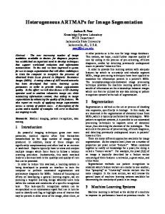
black pixel, and then finally dividing the variable by the number of pixels in the image. This will give the overall proportion of black pixels within the image as a whole. Once we have the average black-pixel density of the image, we can test each section (with a preliminary suggested size of 200*200 pixels), to see if it has a greater than average density of black pixels. This scanning will start at all four corners of the image, simultaneously, and work towards the centre. Once a section of pixels with a greater than average density has been located, we will check that the density of the 3 adjacent sections, connected relatively inward, also have a greater than average density of black pixels. If this is the case, the initial section marks a corner of our area-of-interest. If not, the algorithm will move on the next section. Area of interest detection has been implemented as per the initial design, following Figure 2.3. We first of all split the image into n x m blocks of size s, and launch 4 threads, with starting points (0,0), (0,n), (m, 0) and (m, n). These threads then converge centrally, comparing the density of black pixels in each section. The algorithm, then calculates the dimensions of the bounding box required to hold all 4 detected sections, and returns this as a java Rectangle for use in the line segmentation algorithm.
Figure 2.3: Area of Interest Detection algorithm detects the primary block of text in a manuscript by searching for groups of pixels with lower than average levels of whitespace in an inward-relative direction.
A graphical representation of this process is shown in Figure 2.3, where the arrows show the starting points and directions of travel, the green boxes show the first detected sections, and the grey boxes show the 3, relatively central, sections, which must also meet the greater than average black pixel density criteria. The area of interest would be the bounding box which encompasses all 4 green sections.
2.1.7
Line Segmentation
Due to its need to detect alternating areas of black and white pixels in one continuous area, LineSegmenter is the only algorithm which can not easily be multithreaded. This does not have a massive performance implication though, since LineSegmenter has far less operations than most other algorithms, and most of these operations are purely mathematical. LineSegmenter operates in 3 primary stages. The first is to calculate the density of black pixels on each row of pixels within the image, and finally take the average of these lines. Next, the algorithm searches for lines of text. This is performed by searching for a row of pixels which has a greater than average density of black pixels. Once this is found at y, y − 1 is marked as 15
the opening point of a line. The search then changes to look for the first row of pixels which has a less than average density of black pixels, and again, once this is found at y, y − 1 is marked as the closing point of a line. This process repeats until the end of the area of interest is reached, as shown in Algorithm 5. Algorithm 5 Line Segmentation within Area of Interest size w*h 1: def lines ← new array of (y1 , y2 ) 2: for y from 0 to h − 1 do 3: for x from 0 to w − 1 do 4: if color(x, y) == BLACK then 5: y1 ← y 6: for i from x to h − 1 do 7: for j from 0 to w − 1 do 8: if color(i, j) 6= BLACK AND i == w − 1 then 9: y2 ← j − 1 10: lines ← lines + (y1 , y2 ) 11: x←i+1 12: go to 16 13: end if 14: end for 15: end for 16: end if 17: end for 18: end for
The final stage of the algorithm is to verify the integrity of the detected lines. This is done by firstly matching opening values of y to their corresponding closing values. Each opening y is then compared to the previous opening y, and if the distance between them is less than half of the average distance between lines, the line is deleted. The remaining lines are then converted into rectangles with the same width as the area of interest. This list of rectangles are then returned for use in the next stage in the process.
2.1.8
Letter Segmentation
Letter segmentation is the most complicated of the stages. Letters are segmented by following the same method as Line Segmentation (Section 2.1.7), scanning horizontally as opposed to vertically, along each individual detected line. The overall letter segmentation is performed in 4 stages: Initial Segmentation Letters are segmented, as above, with the image thresholded at the level given by the user in the process panel. This process is outlined in Algorithm 6. Small Letter Joining Once the letters have been segmented, the segments are analysed. Any sequential segments which are both less than half the average width in size, and close to each other, are merged. These merged segments are then re-segmented, using an image which was thresholded at a 16
Algorithm 6 Letter segmentation within Area of Interest size w*h and array of lines L 1: def letters ← new array of (x1 , x2 ) 2: for i from 0 to L.size − 1 do 3: lineopen ← L[i].y1 4: lineclose ← L[i].y2 5: for x from 0 to w − 1 do 6: for y from lineopen to lineclose do 7: if color(x, y) == BLACK then 8: x1 ← x 9: for i from x to w − 1 do 10: for j from lineopen to lineclose do 11: if color(i, j) 6= BLACK AND j == lineclose then 12: x2 ← i − 1 13: letters ← letters + (x1 , x2 ) 14: x←i+1 15: go to 20 16: end if 17: end for 18: end for 19: end if 20: end for 21: end for 22: end for higher level (resulting in thicker lines/more noise), in an attempt to join any letters which were split by the segmentation process. This is shown graphically in Figure 2.4.
Figure 2.4: The Effect of Re-Segmenting using Differing Threshold Levels
Large Letter Splitting Once any small letters have been joined as necessary, a similar process is performed for any letters that are larger than average (thus having a width > 2 ∗ average). Any letters which meet this criteria are re-segmented using a darker image, which highlights any gaps between letters, allowing the segmented to detect the gap if one exists. Again, this is shown in Figure 2.4.
17
Fine Adjustment The final stage of the process is to fine-tune the height of each segment to the height of the letter. To do this, each individual box is expanded vertically, in both directions, until either whitespace is met, or the expansion reaches the 150 pixel limit. This 150 pixel limit has been put in place to ensure that the segmenter doesn’t detect the line below as part of the letter, which would result in a continuously expanded box (in rare circumstances this could occur such as the tail of a y meeting the head of a d).
2.2
Data Structures
As shown by the Class Diagrams given in Appendix X, the system uses 3 primary data structures - Manuscript Library, which holds a collection of Manuscripts, which, in turn, contains a collection of Letters.
2.2.1
Manuscript Library Data Structure
The Manuscript Library data structure is the simplest of the 3, containing one single variable, an enumerated LinkedList, initialised to hold Manuscript objects. Methods are provided to add and remove manuscripts to and from the library, and it is possible to retrieve manuscripts based on their filename and label. This uses a very basic search method - iterating over all manuscripts in the list, returning the first that matches the given string (as shown in Figure 2.5). public Manuscript getManuscriptByFilename(String filename) { for(Manuscript m : getManuscripts()) { if(m.getFilename().equals(filename)) { return m; } } return null; } Figure 2.5: Getting a Manuscript from the Library
In order to reduce the memory footprint of the system, the LinkedList variable is not initialised at runtime, and is instead uses lazy instantiation. The variable is initialised upon the first call to the getManuscripts() method.
2.2.2
Manuscript Data Structure
The Manuscript structure contains information about a particular manuscript (or image), and an enumerated LinkedList of Letters that the manuscript contains. The Manuscript data structure contains the filename, label, notes, import and process dates of the image itself. It also stores the algorithmic parameters used for the blur, padding and threshold stages of the process, the last time the image was processed. The class contains several methods for finding and manipulating letters, including getLetterAtPoint(x, y), which returns the letter visible at any given coordinate (Figure 2.6), and similar methods to the Manuscript Library class, for getting letters by their label. The class also has a 18
method which allows the user to check if a Manuscript already contains a given letter. Whilst not all of these methods have been used in the devised algorithms, the data structures have been designed to be as structurally sound as possible, providing an adequate grounding for future development. public Letter getLetterAtPoint(int x, int y) { for(Letter l : getLetters()) { if(l.contains(x, y)) { return l; } } return null; } Figure 2.6: Finding the Letter at any given Point This is done by iterating through the list of Letters, and checking if the bounding box of each letter contains the given point (this method is later referred back to the native java Rectangle class.
2.2.3
Letter Data Structure
The Letter structure stores information about individual letters, including their label, any notes about them, their coordinates, and whether or not they have been flagged for review. To allow easy reference without having to perform reverse searching, it also stores a reference to the Manuscript in which the Letter is contained. Coordinates are stored as two java Point objects, with one storing the top left (start) point of the bounding box of the letter, with the other storing the bottom right (end). This approach was chosen since it is more flexible than using a java Rectangle when it comes to manupulation. As an example, extending the bounding box upwards by 1 pixel using points could be completed using the function call startCoordinate.setY(startCoordinate.getY() + 1). The same transformation using java Rectangle would require 4 effective operations over 2 function calls - one to set the position (both x and y), and one to increase the size (again, both width and height). The Letter class also contains several other manipulation and searching methods, including a direct method which will resize the letter in any direction, by moving the corresponding Point as previously described. public boolean contains(int x, int y) { if(x > getStartCoordinate().getX() && x < getEndCoordinate().getX()) { if(y > getStartCoordinate().getY() && y < getEndCoordinate().getY()) { return true; } } return false; } Figure 2.7: Checking if a Point (x,y) is within the Boundary Box of a Letter
19
The contains(x, y) method is also available, which checks if the point (x, y) is contained within the bounding box dictated by the two Point objects. This method is shown in Figure 2.7. The class also allows direct comparison with other letters, based on the label and notes of the two letters, as shown in Figure 2.8. public boolean isSimilarTo(Letter otherLetter) { if(!getLabel().equals("Unknown Letter") && getLabel().toLowerCase().equals(otherLetter.getLabel().toLowerCase())) { return true; } else if(!getNotes().equals("No Notes") && getNotes().toLowerCase().equals(otherLetter.getNotes().toLowerCase())) { return true; } else { return false; } } Figure 2.8: Comparison of Letters using Labels and Notes
20
Chapter 3
Experimental Results 3.1 3.1.1
Segmentation Progress Segmentation Process & Results
The segmentation process has achieved a letter recognition accuracy of approximately 90% (as shown in Appendix VI) within images which have not suffered an damage. On noisier images, the result is slightly lower, but remains above 80% in most cases. Figures 3.1 and 3.2 (AOI Detection) show the stages of the process in succession. Firstly, all colour is removed from the image, followed by blurring of the image, to soften the colour harshness of any small areas of noise. Once the image is blurred, it is then thresholded, at the level set in the UI (Figure 3.1 shows thresholding at 105).
Figure 3.1: Segmentation Process: shows the image at various points of the segmentation process. From top to bottom: colour removed, blurred, thresholded, lines segmented, and the final letter-segmented image. The area-of-interest (run between thresholding and line segmentation) is shown separately in Figure 3.2.
Once the image is thresholded, the area of interest is detected (Figure 3.2), which highlights the section of the image most likely to contain letters. This eradicates noise around the edge of the image resulting from the scanning process. This area of interest is then scanned for rows of text (Figure 3.1), and then, in turn, each row of text is then scanned for individual letters. Once the letters have been found, each individual letter is adjusted in an attempt to find its best fit. The resulting output can be seen in the final row of Figure 3.1.
21
Figure 3.2: Segmentation Process: Area of Interest Sample Output This process is able to detect the vast majority of letters within manuscripts, even if high levels of noise are present. Since the algorithm is very much heuristic, adjustments can be made in the user interface, through the use of keyboard shortcuts. In order to aid this finishing process, any letters which the algorithm determines to be anomalous post-segmentation are automatically flagged for review, meaning that they will be coloured red. This is determined by validating the width of the letters, since prior knowledge of the manuscripts in question shows that the vast majority of letters are of an approximately equal width. An example of a segmented manuscript is shown in Appendix VII.
3.1.2
Effect of Parametric Setting Adjustments
Both the Thresholder and Blurrer algorithms allow the user to adjust their parameters. For thresholding, this is the colour level at which the colour becomes white. In blurring, it is the radius around each pixel which is taken into account when blurring the image. The values of these parameters are crucial in the success of the segmentation process.
Figure 3.3: Effect of Threshold Level Adjustment. From top to bottom: Original Image, Thresholding at 64, Thresholding at 96, Thresholdng at 128, Thresholding at 160, Thresholding at 192.
The threshold level is adjustable from 0 (where only black pixels remain black) to 255 (at which point all pixels will become black). Figure 3.3 shows the effect of various threshold levels on a section of one of the manuscripts used for evaluation purposes. The first row of text is the original image, with the lines below showing the result of thresholding from 64 to 192, at intervals of 32. At 192, the vast majority of the image is black, and thus no text is distinguishable, whilst at 160, text becomes readable, but there is still a large amount of noise.
22
The levels of noise become acceptable at 128, with the only remaining noise being black bars to the left and right, which would be removed by the area of interest detector. The differences between 64 and 128, whilst seemingly minor, are actually the variances which make the most difference to the letter segmentation process. For example, looking at the final two letters on the second word, ”ad”, at 128 they are clearly joined. Upon reducing the threshold level to 64, however, the join between them isn’t dark enough to withstand the thresholding, and they become two distinct letters. This shows the reasoning behind thresholding 3 times in the process - we threshold at an average, middle ground, level, suggested by the user, and then use a lower level to detect letters which should be split, and then a higher level to join letters which have been mistakenly split when thresholded at the original level. This process ensures that the majority of letters are detected correctly, and, compared to using a single threshold level, results in a roughly 30% increase in the proportion of accurately detected letters. The second adjustable parameter, the blur radius, is adjustable in the range m = [0, 10]. The decision to limit this to such a small range is due to the running time of the algorithm, O(nm2 ). Blurring removes smaller objects of noise by reducing their colour levels, resulting in them being coloured white by the thresholding algorithm. An example of this is shown to the far end of the line of text in Figure 3.4. To the right of the final ”L” are two very small dots of noise. As the blur radius increases, these dots get lighter until, when blurring at a radius of 10px, they are not longer visible.
Figure 3.4: Effect of Blur Level Adjustment. From top to bottom: Original Image, Blurring at 1px, Blurring at 5px, Blurring at 10px, Blurring at 25px.
Figure 3.4 shows why the ColorRemover algorithm must be run first. Due to the colour of the paper on which most manuscripts are presented, blurring the image increases the effect of this greater than average red level, and the entire image takes a red tint. Removing the colour from the image, however, does not affect the Blurrers ability to remove noise from the image, and also stops these high red levels from affecting the Thresholder.
3.2 3.2.1
Technical Performance Resource Usage
The system will fully utilise as much CPU processing power as the computer has available, and is set to, by default, run within a 2GB java memory heap. During testing, on a Mac OS X system, after processing 20 images of resolution 4000x6000 pixels in quick succession, memory usage remained below 1GB. Memory usage below this would be difficult to achieve, due to how Java keeps BufferedImages in memory whilst they are being iterated over.
23
3.2.2
Algorithm Performance
As described in Section 3.2.3, all algorithms are multithreaded to increase performance levels, with the exception of LineSegmenter. All designed algorithms run in linear time, with the exception of the Blurrer algorithm, which runs in O(nm2 ), where n is the pixel count, and m is the blur radius. This performance is reasonable with small values of m, thus m is limited to values ≤ 10 in the GUI. With the default blur radius value of 1, the entire process occurs in linear time, with respect to the number of pixels and letters present in the image. It would be valid to say that the segmentation process runs in O(lm2 n), where l is the number of letters present in the image, m is the blur radius selected and n is the number of pixels. It is important to note that the algorithms developed are heuristic, in that they do, in no way, guarantee an optimal result. The algorithmic parameters are key to the system’s success whilst the system will predict the best thresholding level to use, it is important for the user to use their judgement - since certain aspects can skew this prediction. If the image, for example, has large dark areas to the top or bottom (or anywhere away from the main block of text), this may lower the predicted threshold value, which may skew the overall result. With optimal threshold settings, on average, the system detects approximately 90% of letters within a manuscript, excluding any which have been the subject of paper damage.
3.2.3
Effectiveness of Parallelisation on Running Time
All algorithms use a dynamic number of threads, matching the number of available CPU cores on the system, to process several parts of the image simultaneously. The exceptions to these are LineSegmenter, which, due to the nature of the algorithm, can only use one thread, and AOIDetector, which always uses 4 threads. Algorithm Blurrer Color Remover Thresholder AOI Detector Line Segmenter Letter Segmenter
No MT 1 1 1 1 1 1
1C 1.037 1.007 0.997 1.38 1.03 0.993
2C 0.553 0.563 0.507 1.187 1.017 0.52
2C (HT) 0.593 0.633 0.54 0.993 0.983 0.533
4C 0.28 0.283 0.277 0.413 0.967 0.267
4C (HT) 0.297 0.303 0.317 0.533 0.967 0.263
Figure 3.5: Average Multithreaded Algorithm Performance (Relative)
Figure 3.5 shows the average performance times of the algorithms, relatively compared to having no multithreading, over various CPU configurations. This is shown in greater detail (including tests with multiple images) in Appendix V. These results show a maximum performance increase of up to 380% (LetterSegmenter running on 4 cores with hyper threading enabled), and also show how some some of the algorithms can have a minor decrease in performance under circumstances. Take, for example, AOIDetector. This algorithm takes 38% and 18.7% longer to run on systems with 1 or 2 cores, compared to running with no multithreading. Once the core count reaches 4 (2 with hyper threading results in 4 virtual cores), we start to see a marginal increase in performance, with the performance increasing dramatically upon reaching 4 physical cores.
24
This minor decrease in performance for the two non-multithreading-optimised algorithms, however, is negated by the much larger increase on the slower algorithms (AOIDetector and LineSegmenter are the two fastest algorithms by nature). On a two core machine, for example, the 18% performance decrease for AOIDetector is outweighed by the increases for the much slower Blurrer and Thresholder, which is run 3 times during the segmentation process.
Figure 3.6: Algorithm Performance Graph. HT = Hyper Threading.
The performance of each algorithm over each configuration is graphed in Figure 3.6, with a polynomial trend line. This graph shows that whilst LineSegmenter remains fairly stable in its running time over all configurations, the running time of each algorithm is inversely proportional to the number of cores available (all show a downward trend). For LineSegmenter, which is not multithreading aware, this slight performance gain is most likely attributed to enhanced operating system performance with multiple cores (since it will have a full core available, instead of one core minus operating system resources), and the ability of Java to offload its own threads (such as the GUI objects) over multiple cores, thus freeing up resources. The graph shows, however, there is sometimes a slight performance decrease when hyperthreading is used. This can be attributed to java not being hyper-threading aware, and reporting the number of virtual CPU cores, as opposed to physical. This results in splitting the same work, over the same number of physical cores, twice as much, meaning that each core has to juggle two simultaneous jobs. As of the current Java version, there is no way to retrieve the number of physical cores, and even with this negligible performance decrease, the performance increase given between configurations is worthwhile.
25
Chapter 4
Conclusions & Future Research 4.1
Conclusions
4.1.1
Performance
The system achieves high levels of performance, and reasonably high rates of success at detecting letters within manuscripts. By dividing the problem, the system is able to achieve linear time performance (dependant on the blur radius setting given by the user), and thus, depending on the host computer, is able to detect upwards of 1000 letters in a manuscript in 15-30 seconds. Comparing this to manual annotation, if a palaeographer was able to annotate one letter every 3 seconds, and worked continuously, the same task would take approximately 50 minutes - up to 200 times longer.
4.1.2
Noise Removal
Noise removal takes place in several stages, thresholding removes the majority of noise, whilst blurring the image removes minor groups of pixels which could affect the segmentation algorithm. Any exterior noise not removed by these methods is then filtered out when the area of interest is detected. Instead of wasting time attempting to remove high amounts of noise around the edges of the image, the algorithm adapts to ignore this area, and focus on areas with a greater than average density of black pixels, in a pattern which suggests text is present.
4.1.3
User Interaction
Whilst the system is able to automatically suggest thresholding levels based on average colour levels within the image, it allows the user to easily customise the process. It also allows the user to change how letters are displayed, by setting padding levels, improve the detection of letters by adjusting the thresholding level (since the user can take into account visual artefacts), and the amount of blurring that takes place. This also provides a way for the user to adjust how long the process takes - since higher levels of blurring can make noise removal more reliable, but also substantially increases the running time as the blurring algorithm runs in quadratic time. High levels of usability have been maintained in the GUI - ensuring all use cases are easy to perform. No operation takes more than 4 mouse clicks, and the most commonly required features have been prominently placed as buttons on the main screen. The image library is fully searchable, which allows the user to maintain a large library of images without decreasing usability. Several smaller functions have also been implemented, such as printing support, and
26
the ability to handle deleted images without having to resort to manually deleting files from within the operating system.
4.2 4.2.1
Future Research & Extensions K-Means Clustering Implementation
Although the current letter adjustment algorithm is fast, and achieves relatively high levels of accuracy, it could be improved through the use of K-Means Clustering. K-Means Clustering was not implemented in this project for two reasons - firstly, it would increase the complexity of the programming required dramatically, thus delaying the project. Secondly, and more importantly, it would increase the asymptotic running time of application to extremely high levels. With further research, however, this could be implemented in reasonable time. One example of how this would be possible is to follow the approach that this entire project has taken divide and conquer. Instead of performing one large clustering run on the entire image, with each known letter to be a mean, one could perform clustering around each individual letter, or group thereof, only including pixels within a certain radius of each letter.
4.2.2
Artificial Intelligence
Another way in which the system could be improved with further work is through the use of artificial intelligence. The system, in its current state, is dumb, in that it doesn’t learn from its mistakes or user actions. The system could, for example, learn about thresholding levels on different styles of images based on the post-processing adjustments that the user makes. An example of this in practice would be that if the user adjusts a large proportion of detected letters to be taller, the letter segmentation algorithm needs to be adjusted when run on similar images. This could also be a great benefit to the threshold prediction function, which currently performs a linear operation on the average colour within the image. The system could learn which threshold levels achieve best performance on images with differing characteristics, thus using this information to improve its prediction.
4.2.3
Interaction with Existing and Future Tools
One of the key areas of extension, however, is the system’s ability to interact with other tools. Since the system both reads from, and saves to, a library file in standards-compliant JSON format, it is perfectly possible for other systems to read data from this file. Take, for example, an OCR system which is capable of very high identification rates of individual letters. Such a system could read each letters coordinates from the JSON file, attempt to detect the letter, and feed this information back into the JSON file. This would allow this system to automatically identify the detected letters without further programming. A further extension of this concept would be to expand the file formats which the system is capable of using - since JSON is still a fairly rare format. The system could, in theory, use a library formatted in XML, CSV, or SQL, allowing an even wider range of systems to interact.
27
Chapter 5
References [1] DigiPal, 2012. Digital Resource for Palaeography. [online] Available at: [Accessed April 2012] [2] Tony Jebara Columbia University, 2000. The Sobel Operator. [online image] Available at: [Accessed April 2012] [3] Northern Kentucky University, 2003. Light Contrast Illusions. [online image] Available at: [Accessed April 2012] [4] Pal, N. R. and Pal, S. K., 1993. A Review on Image Segmentation Techniques. Pattern Recognition, 26(9), pp.1277-1294. [5] Gonzalez, R. C. and Woods, R. E., Digital Image Processing. 3rd ed. Prentice Hall [6] Lee, J., 1983. Digital image smoothing and the sigma filter. Computer Vision, Graphics and Image Processing, 24(2), pp. 255-269. [7] Gull, S. F. and Daniell, G. J., 1978. Image reconstruction from incomplete and noisy data. Nature, 272, pp. 686-690. [8] Cheriet, M., Said, J.N. and Suen, C.Y., 1998. A recursive thresholding technique for image segmentation. Image Processing, IEEE Transactions on, 7(6), pp. 918-921. [9] Wagstaff, K., Cardie, C., Rogers, S. and Schroedl, S., 2001. Constrained K-means Clustering with Background Knowledge. Proceedings of the Eighteenth International Conference on Machine Learning, pp. 557-584. [10] Bradley, P. S. and Fayyad, U. M., 1998. Refining Initial Points for K-Means Clustering. Proceedings of the 15th International Conference on Machine Learning, pp. 91-99. [11] Canny, J., 1986. A Computational Approach to Edge Detection. Pattern Analysis and Machine Intelligence, IEEE Transactions on, 8(6), pp. 679-698. [12] Marr, D. and Hildreth, E., 1980. Theory of Edge Detection Proceedings of the Royal Society of London. Series B, Biological Sciences 207(1167) pp. 187-217. [13] Mumford, D. and Shah, J., 1985. Boundary Detection By Minimizing Functionals. In IEEE Conference on Computer Vision and Pattern Recognition, pp. 22-26. [14] Boyle, L. E., 1984. Medieval Latin palaeography: a bibliographical introduction. University of Toronto Press. [15] Stokes, P. A., 2007. Palaeography and Image-Processing: Some Solutions and Problems. Digital Medievalist. [online journal] Available at [Accessed April 2012] [16] Inaba, M., Katoh, N. and Imai, H., 1994. Applications of weighted Voronoi diagrams and randomization to variance-based k-clustering (extended abstract). Proceedings of the tenth annual symposium on Computational geometry, pp. 332-339. [17] Oracle, 2004. Bug ID: 5082531 JScrollPane and FlowLayout do not interact properly. [online] Available at: [Ac28
cessed June 2012] [18] Soler, L., Delingette, H., Malandain, G., et. al, 2001. Fully automatic anatomical, pathological, and functional segmentation from CT scans for hepatic surgery. Computer Aided Surgery, 6(3), pp. 131-142. [19] Garain, U., Parui, S. K., Paquet, T. andHeutte, L, 2007. Machine Dating of Handwritten Manuscripts. Ninth International Conference on Document Analysis and Recognition, 2, pp. 759-763. [20] Tizhoosh, H. R., 2005. Image thresholding using type II fuzzy sets. Pattern Recognition, 38(12), pp. 2363-2372.
29
Appendix Appendix I: Sample Raw Manuscript Image
CCCC 162, pp. 1 - 138, 161 - 564: 109. The Master and Fellows of Corpus Christi College, Cambridge.
30
Appendix II: Algorithm Data Flow Design
31
Appendix III: JSON Format Example { ’manuscript’ : [ { ’filename’ : ’!CCC111_007v2.jpg’, ’label’ : ’!CCC111_007v2.jpg’, ’notes’ : ’No notes’ ’importdate’ : ’19/07/2012’, ’blur’ : ’0’, ’padding’ : ’0’, ’threshold’ : ’53’, ’processdate’ : ’19/07/2012’, ’letter’ : [ { ’filename’ : ’!CCC111_007v2.jpg’, ’label’ : ’Unknown Letter’, ’notes’ : ’No Notes’, ’flagged’ : ’false’, ’geometry’: { ’type’: ’Polygon’, ’coordinates’ : ’[[1288, 923], [1299, 923], [1288, 930], [1299, 930]]’ }, ’crs’: { ’type’: ’name’, ’properties’: { ’name’: ’EPSG:3785’ } }, ’type’: ’Feature’, ’properties’: { ’saved’: 1 } } ] } } }
32
Appendix IV: Process Panel GUI Screenshot
33
Appendix V: Parallelisation Performance Testing This table shows the relative performance of all algorithms running on various CPU configurations (HT suggests that hyper threading was enabled, and thus the test was using double the number of virtual cores), compared to the algorithm running without multithreading. Testing was conducted in a virtualised Mac OS X 10.7 installation, running on an Apple iMac, with Intel Core i7 2600 CPU (3.4GHz), 32GB RAM (8GB available to the virtual machine) and a solid state drive. All processor core limitations were applied in the used virtualisation software, to ensure that the results were not affected by the use of different specification processors. Algorithm Blurrer
Color Remover
Thresholder
AOI Detector
Line Segmenter
Letter Segmenter
Image 1 2 3 Average 1 2 3 Average 1 2 3 Average 1 2 3 Average 1 2 3 Average 1 2 3 Average
No MT 1 1 1 1 1 1 1 1 1 1 1 1 1 1 1 1 1 1 1 1 1 1 1 1
1C 0.98 1.03 1.01 1.007 1.11 1.03 0.97 1.037 1.01 1.01 0.97 0.997 1.58 1.36 1.2 1.38 0.99 1 1.1 1.03 0.95 0.98 1.05 0.993
34
2C 0.61 0.57 0.51 0.563 0.58 0.53 0.55 0.553 0.53 0.48 0.51 0.507 1.31 1.2 1.05 1.187 1.02 0.98 1.05 1.017 0.5 0.51 0.55 0.52
2C (HT) 0.72 0.6 0.58 0.633 0.59 0.58 0.61 0.593 0.55 0.56 0.51 0.54 1.12 0.95 0.91 0.993 0.97 0.99 0.99 0.983 0.52 0.55 0.53 0.533
4C 0.28 0.26 0.31 0.283 0.26 0.27 0.31 0.28 0.28 0.25 0.3 0.277 0.5 0.41 0.33 0.413 0.95 0.96 0.99 0.967 0.25 0.24 0.31 0.267
4C (HT) 0.3 0.28 0.33 0.303 0.28 0.3 0.31 0.297 0.29 0.31 0.35 0.317 0.61 0.5 0.49 0.533 0.97 0.95 0.98 0.967 0.26 0.28 0.25 0.263
Appendix VI: Segmentation Accuracy Testing Results The following table shows the results of testing the accuracy of the segmentation process. Images were segmented using their optimal values, and the proportion of letters within the image accurately detected, and the number of false detections, were measured. These two measures are independent -Letters Detected represents the percentage of letters detected successfully, whilst the False Positive Rate is the proportion of boxes which detect noise as a letter. Image Image 1 Image 2 Image 3 Image 4 Image 5 Image 6 Image 7 Image 8 Image 9 Image 10 Average
Letters Detected 87% 91% 95% 94% 85% 84% 92% 87% 89% 93% 89.8%
35
False Positive Rate 5% 6% 4% 2% 5% 4% 5% 3% 4% 6% 4.4%
Appendix VII: Sample Segmented Image (Post-Processing)
CCCC 162, pp. 1 - 138, 161 - 564: 109. The Master and Fellows of Corpus Christi College, Cambridge.
36