it feasible to implement the half-octave Gaussian pyramid in embedded computing ..... We have vali- dated our model by comparing a simulation of our random.
Probabilistic Model of Error in Fixed-Point Arithmetic Gaussian Pyramid Antoine M´eler
John A. Ruiz-Hernandez James L. Crowley INRIA Grenoble - Rhˆone-Alpes 655 avenue de l’Europe 38 334 Saint Ismier Cedex France
{Antoine.Meler,John-Alexander.Ruiz-Hernandez,James.Crowley}@inrialpes.fr
Abstract The half-octave Gaussian pyramid is an important tool in computer vision and image processing. The existence of a fast algorithm with linear computational complexity makes it feasible to implement the half-octave Gaussian pyramid in embedded computing systems using only integer arithmetic. However, the use of repeated convolutions using integer coefficients imposes limits on the minimum number of bits that must be used for representing image data. Failure to respect this limits results in serious degradation of the signal to noise ratio of pyramid images. In this paper we present a theoretical analysis of the accumulated error due to repeated integer coefficient convolutions with the binomial kernel. We show that the error can be seen as a random variable and we deduce a probabilistic model that describes it. Experimental and theoretical results demonstrate that the linear complexity algorithm using integer coefficients can be made suitable for video rate computation of a half-octave pyramid on embedded image acquisition devices.
1. Introduction Over the last years, the pyramid and Gaussian derivative features have emerged as a powerful source of image features for computer vision and pattern recognition. Gaussian derivative features have been used for 3D reconstruction, image stitching, object recognition [9] [10] and detection of faces [8] and other categories of image objects. Gaussian derivative features are the basis for SIFT descriptor [7], the histogram of gradients [4] and the second local order structure image solid [6]. Such features are also used in biological vision models [5]. An inconvenience of Gaussian derivative features is that most algorithms require relatively expensive floatingpoint computations with algorithmic complexities of N 2 or worse. It is possible to compute such features with a linear
complexity algorithm using only integer coefficient convolutions. However, the use of this algorithm requires careful attention to the signal noise introduced by roundoff error during repeated convolutions with integer coefficient filters. Crowley and Stern [3] have proposed a linear complexity algorithm for computing an exactly scale invariant Gaussian pyramid using a technique referred to as Cascade convolution with resampling. This algorithm has an O(N ) complexity where N is the number of pixels in the image and produces 2logn (N ) resampled images in which each image has an identical impulse response at a logarithmically increasing set of scales. An integer coefficient version of this algorithm, the halfoctave binomial pyramid was proposed by Crowley and Riff [2] in 2003. A pyramid computed with this algorithm can provide Gaussian derivative image features using only simple sums and differences of pixels. As a result, this algorithm is suitable for calculation of Gaussian derivative features on embedded computing devices. However restrictions in the available memory on such devices can lead designers to implement the algorithm with as few as 8 bits per pixel. When used with repeated convolution, this a restricted bit length introduces serious degradation in the signal to noise ratio of the resulting pyramid. Such errors can cause important loss of reliability and precision of image descriptors based on the pyramid. In this paper we present a probabilistic model for the error resulting from the computation of the half-octave Gaussian pyramid fixed point integer coefficients. This model describes the error generation and propagation at each pyramid level due to recursive convolutions with a binomial kernel. Our results show that the half-octave pyramid can be accurately computed with short fixed-point numbers. This paper is organized as follows. Section 2 explains the half-octave Gaussian pyramid algorithm. Our probabilistic error model is developed in section 3, followed experimental verification in section 4. Section 5 concludes with discussion of the results and its application for embedded image processing.
Image
σ=8 √ σ=4 2
2D Binomial Convolutions
σ=4 √ σ=2 2
2D Binomial Convolutions σ=2
√
2 Resampling
Level 1
Pyramid Buffer
derivation
Pyramid Derivative
σ=
√
2
2D Binomial Convolutions l =l+1 √
2 Resampling
Level l
Figure 2. The half-octave pyramid algorithm result Figure 1. The O(N) cascade convolution pyramid computation scheme
...
2. The Half-Octave Gaussian Pyramid In this section we describe the calculation of the halfoctave Gaussian pyramid and its derivatives. A linear complexity pyramid algorithm for the calculation of Gaussian derivatives has been known since the 1980’s [1] (figure 1). This algorithm involves alternatively convolving with a Gaussian support, and resampling the resulting image. The result of this algorithm is a half-octave Gaussian pyramid. An integer coefficient version of this algorithm [2] has been demonstrated using repeated convolutions of the binomial kernels [1, 2, 1] and [1, 2, 1]t . Implementations that compute such pyramids on PAL sized images and bigger exist for the current generation of computer stations, and can be embedded in dedicated signal processor. The half-octave Gaussian pyramid for an N ∗ N pixels image is composed of up to L = 2 log2 (N ) images. The effect of cascade convolution is to sum the variances of the filters, so that the cumulative variance for the image l ∈ [[ 1, L ]] is σl = 2l . That for, the convolution step involves 2 convolutions by [1, 2, 1] in each direction. Interleaving resampling with convolutions decreases the number of image samples while expanding the distance between samples. This has the effect of dilating the Gaussian support without increasing the number of samples used for the Gaussian, effectively increasing the scale. The resampling rate is set to √ 2, resulting in a constant ratio of scale over sample distance. The resulting pyramid represents the original N ∗ N pixels image with a sequence of 2 log2 (N ) images at a geometric progression of scales each with twice as less samples as the previous, resulting in a total of 2N 2 samples (figure 2). The 2-dimensional derivative of order (dX , dY ) is then obtained by convolving dX times the resulting pyramid with the derivative kernel [−1, 0, 1], and dY times with [−1, 0, 1]t .
x ˜k−1 (i, j)
x ˜k (i, j)
x ˜k+1 (i, j)
�2
�1
�2
...
...
x ˜k−1 (i, j)
x ˜k (i, j)
�1
x ˜k (i + 1, j)
...
�1 −
+ ...
x ˜k+1 (i, j)
...
...
x ˜k (i, j + 1)
(a)
...
(b)
Figure 3. Convolution with the two base kernels (smoothing (a) and differentiation (b) ) . The � n operator stands for right n bits shift with zero padding
3. Probabilistic Formulation 3.1. Random Error Model In this section, we present our model to analyze the noise effect of using fixed point coefficients for the pixel values in the pyramid. Let x ˜~k (~i, ~j) be the value of the pixel of coordinate ~k after ~i smoothing convolutions and ~j differentiations in directions X and Y. x ˜~k (~i, ~j) is the sum of an exact theoretical ~ ~ value x~k (i, j) and an error E~k (~i, ~j). x ˜~k (~i, ~j) = x~k (~i, ~j) + E~k (~i, ~j)
(1)
We model the error E by a random variable. In order to simplify the problem, the error part of contiguous pixels is supposed independent. This approximation is verified to be very accurate in section 4. Thus, we will simply consider E(i, j) where i and j are the number of smoothing and differentiation convolutions respectively applied to one pixel, including both directions X and Y. We consider only two operations: convolution with the normalized kernels Ks = [ 14 , 12 , 14 ] and with Kd = [ 12 , 0, − 12 ] as schematized on figure 3. We also suppose that all the convolutions with Ks are applied before those with Kd . Thus, we express E(i, j = 0) as a function of E(i − 1, j), then E(i, j > 0) as a function of E(i, j − 1).
3.2. Error Generation and Propagation
3.3. Total Accumulated Error
x ˜ is a fixed point number with ni bits of integer part and nf bits of fractional part. Furthermore, x ˜ is supposed to be initially an integer (i.e. its nf least significant bits are 0) . Because pyramid computation is recursive, the error of one value is composed of two parts. One is a new error, generated by the current computation E new , and the other, E prop , is accumulated during the previous computations and propagated to the new value. In this section, we determine, for a given number of fractional bits nf , the expressions of the random variables Ennew f and Enprop . f
The total error is the sum of the propagated part and the generated part:
Error generation Ennew is the error generated by the calf culation of a new pyramid value. As shown in figure 3, a convolution with Ks or Kd starts with divisions by a number 2nshif t , which, in fixed point arithmetic, corresponds to a bit shift with the loss of the nshif t least significant bits. Such a division can be modeled with UVnf (nshif t ) , the uniform discrete random variable � with the set of possible values Vnf (nshif t ) = � −i . In the case of values being 2nf +nshif t i∈ [ 0,2nshif t −1 ] initially integers, this model is well-suited for 2i + j > nf . Before this condition is true, the divisions do not lead to a loss of information. Thus, the generated error is equal to:
Enf (i, j) = Enprop (i, j) + Ennew (i, j) f f
We deduce from the above model the error characteristics (standard deviation and variance) as a function of the number of smoothing convolutions (i) and differentiations (j). We first express the error with recurrence formulation, and then give the solution. Error evolution The values are initially integers, Enf (i, j) = 0 for 2i + j ≤ nf . Thus we express the expected value E[Enf (i, j)] and the variance V ar[Enf (i, j)] of the complete error random variable for 2i + j ≤ nf . In this condition, Enprop (i, j) and Ennew (i, j) can be supposed f f independent. Smoothing convolutions are computed before computing image derivatives from image differences. Thus we first give the recurrence law for smoothing (j = 0) and then for derivative computation (j > 0). • Smoothing: h i h i new E[Enf (i, j = 0)] = E Enprop (i, j) + E E (i, j) nf f � � 1 = E Enf (i − 1, j) − nf 2
• If 2i + j ≤ nf : Ennew (i, j) = 0 f
(2)
=
Ennew (i, j = 0) = UVnf (2) + UVnf (1) + UVnf (2) f (i, j > 0) = UVnf (1) − UVnf (1) Ennew f
� � 5/3 3 V ar Enf (i − 1, j) + (2n +5) 8 2 f
(7)
• Derivation: (3)
Error propagation This paragraph considers the error that propagates from a state (i, j) to the next (i + 1, j) or (i, j + 1). We assume the number of integer bits, ni , is sufficient to avoid overflow. In this case, the error Enprop (i, j) propf agated during a convolution with Ks or Kd is a random variable defined by recurrence: prop Enf (0, 0) =0 E prop (i, j = 0) = Enf (i−1,j) + Enf (i−1,j) nf 4 2 Enf (i−1,j) + 4 En (i,j−1) En (i,j−1) prop Enf (i, j > 0) = f 2 − f 2
(6)
h i h i new V ar[Enf (i, j = 0)] = V ar Enprop (i, j) + V ar E (i, j) nf f
• Otherwise: (
(5)
h i h i E[Enf (i, j > 0)] = E Enprop (i, j) + E Ennew (i, j) f f =0
(8)
h i h i (i, j) + V ar Ennew (i, j) V ar[Enf (i, j > 0)] = V ar Enprop f f =
� � 2/3 1 V ar Enf (i, j − 1) + 2(n +2) 2 2 f
(9)
Error expression We can deduce the absolute expressions of E[Enf (i, j)] and V ar[Enf (i, j)] as a function of i, j and nf . (4) � E[Enf (i, j)] =
−1 2nf
0
i−
nf 2
�
if j = 0 otherwise
(10)
level 1, 2nd derivative
level 1
V ar[Enf (i, j)] =
1 1 3
nf
i− 2 − 38 22nf +j+2
�
+
� (11)
j 1 − 12 22nf +2
Note that the error variance increases with i and j toward a limit: V ar[Enf (∞, 0)] = V ar[Enf (i, ∞)] =
1/3
simulation synthetic photographies
simulation synthetic photographies
-0.45 -0.4 -0.35 -0.3 -0.25 -0.2 -0.15 -0.1 -0.05
0
-0.04
level 6
-0.02
0
level 6, 2
nd
simulation synthetic photographies
0.02
0.04
derivative simulation synthetic photographies
22nf +2
4. Experiments and validation In this section we compare the error predicted by our model with the one measured by subtracting an image pyramid with varying precision (0 ≤ nf ≤ 12) and a 64 bits one. We perform this analyse on synthetic images (Perlin noise) and photos randomly downloaded from the internet.
-0.45 -0.4 -0.35 -0.3 -0.25 -0.2 -0.15 -0.1 -0.05
0
-0.04
-0.02
0
0.02
0.04
Figure 4. Distribution of the error of the pyramid values with nf = 6. abscissa: error value, ordinate: pixel rate with this error.
4.1. Error Distribution To validate our model, we compare predicted and measured error. There is no simple mathematic expression for the distribution of the error as modeled in this paper. However we can estimate it as accurately as needed by running simulations of our random variable. As shown figure 4, our model accurately matches the error distribution measured in pyramids built from highlyinformative images like Perlin noise. In the case of photographies, an unpredicted null-error peak can be observed. The figure 5 demonstrates that in homogeneous areas (sky, unfocused background, over/under-exposition, ...), smoothing convolutions do not alter pixel values which thus stay integers. In such areas, our model for the loss of information as an addition by a random uniform variable fails while the pyramid level is under the singular zone characteristic scale. Thus, our theoretical analysis provides information about the accumulated error in the worst case. One can also observe a larger spread in the measured distributions than in the theoretical one. This difference is due the independence hypothesis which underestimate the variance by neglecting a positive covariance term. However, it appears that this term play a minor part.
(a)
(a’)
(b)
(b’)
Figure 5. Over-exposed photography (a) and associated error image at pyramid level 3 with nf = 6 (a’). The saturated area corresponds to a null-error area which is very poorly modeled by our random error variable. Perlin noise (b) and its associated error image (b’).
4.2. Error Parameters
5. Conclusion
In this section, we graphically display the parameters of the random error variable. Due to the presence of homogeneous areas in photos, experimental standard deviation and variance are very datadependant. It is thus more interesting to visualize the theoretical values which correspond to the worst case (figure 6). It can be seen that the standard deviation convergence in the levels is quite fast. We thus can simply study the limit value (figure 7).
This paper has presented a model for the error due to recursive truncations by a random noise in computing a Gaussian pyramid using a linear complexity algorithm involving cascaded convolution with integer coefficient binomial filters. This model predicts the additive image error as a function of the number of fractional bits used, the scale of the pyramid and the order of the derivative. We have validated our model by comparing a simulation of our random variable and measurements performed in pyramids applied
tion of the pyramid scale. However, the divergence is constant and grows rapidly for small numbers of fractional bits in the fixed point representation. This divergence becomes zero when the signal is differentiated, thus making it irrelevant for many applications. We can conclude by observing that binomial convolution kernels tends to smooth the error noise, thus compensating for random noise added by integer truncation in cascade convolution. This makes the Gaussian binomial pyramid a good multi-scale image representation solution for use in embedded computer vision systems.
Expected Value Standard Deviation 2 1.5 1 0.5 0 0 1 2 6 4 3 4 2 level 5 6 7 8 90
8
12 10 nf
References
(a)
Expected Value Standard Deviation 0.3 0.25 0.2 0.15 0.1 0.05 0 0 1 2 6 4 3 4 2 level 5 6 7 8 90
8
12 10 nf
(b) Figure 6. Expected value and standard deviation of the error variable as a function of the level and the number of fractional bits nf before differentiations (a) and after 2 differentiations (b).
0.3 standard deviation’s limit 0.25 0.2 0.15 0.1 0.05 0 0
1
2
3 nf
4
5
6
Figure 7. Limit value of the error standard deviation as a function of the number of fractional bits nf .
to synthetic images and photos. We have shown that the noise variance rapidly converges to a fixed value as a func-
[1] J. Crowley and A. Parker. A representation for shape based on peaks and ridges in thedifference of low-pass transform. IEEE PAMI, 6(2):156–169, March 1984. 2 [2] J. Crowley and O. Riff. Fast computation of scale normalised gaussian receptive fields. pages 584–598, 2003. 1, 2 [3] J. Crowley and R. Stern. Fast computation of the difference of low-pass transform. PAMI, 6(2):212–222, March 1984. 1 [4] N. Dalal and B. Triggs. Histograms of oriented gradients for human detection. IEEE CVPR, pages 886–893, June 2005. 1 [5] M. A. Georgeson, K. A. May, T. C. Freeman, and G. S. Hesse. From filters to features: scale-space analysis of edge and blur coding in human vision. Journal of vision, 7(13), 2007. 1 [6] L. Griffin. The second order local-image-structure solid. IEEE PAMI, 29(8):1355–1366, 2007. 1 [7] D. G. Lowe. Distinctive image features from scale-invariant keypoints. International Journal of Computer Vision, 60:91– 110, 2004. 1 [8] J. A. Ruiz Hernandez, A. Lux, and J. L. Crowley. Face detection by cascade of gaussian derivatives classifiers calculated with a half-octave pyramid. IEEE Conference on Automatic Face and Gesture Recognition, Amsterdam, Sep 2008. 1 [9] B. Schiele and J. Crowley. Recognition without correspondence using multidimensional receptive field histograms. International Journal of Computer Vision, 36:31–50, 2000. 1 [10] J. Yokono and T. Poggio. Oriented filters for object recognition: an empirical study. In Proceedings of the IEEE FG2004. Seoul, Korea, page 755, 2004. 1