Probability Models for Information Retrieval based on ...

Probability Models for Information Retrieval based on Divergence from Randomness

Giambattista Amati Thesis submitted for the degree of Doctor of Philosophy, Department of Computing Science Faculty of Information and Mathematical Sciences University of Glasgow June 2003

c Giambattista Amati

Glasgow, 3rd June 2003

ii

Abstract This thesis devises a novel methodology based on probability theory, suitable for the construction of term-weighting models of Information Retrieval. Our term–weighting functions are created within a general framework made up of three components. Each of the three components is built independently from the others. We obtain the term– weighting functions from the general model in a purely theoretic way instantiating each component with different probability distribution forms. The underpinning idea on which we are able to systematically construct the term– weighting models is based on the notion of divergence from randomness. The leading theme of the divergence-from-randomness approach is that the informative content of a term can be measured by examining how much the term-frequency distribution departs from a “benchmark” distribution, that is the distribution described by a random process. Following this idea, the first two components of the framework provide an explanation to the duality existing in Information Retrieval between the distributions of topic–terms in a small set of documents (the elite set of a topic) and in the rest of the collection. The third component deals with the term-frequency normalization and is able to compare term frequencies within documents of different lengths. As a consequence, different probability distributions can be used in the framework of the divergence-from-randomness approach. Our experiments utilise some of them to show that the framework is sound and robust and generates different but highly effective Information Retrieval models. The thesis begins with investigating the nature of the statistical inference involved in Information Retrieval. We explore the estimation problem underlying the process of sampling. De Finetti’s theorem is used to show how to convert the frequentist approach into Bayesian inference and we display and employ the derived estimation techniques in the context of Information Retrieval. i

ii We initially pay a great attention to the construction of the basic sample spaces of Information Retrieval. The notion of single or multiple sampling from different populations in the context of Information Retrieval is extensively discussed and used throughout the thesis. The language modelling approach and the standard probabilistic model are studied under the same foundational view and are experimentally compared to the divergence-from-randomness approach. In revisiting the main information retrieval models in the literature, we show that even language modelling approach can be exploited to assign term-frequency normalization to the models of divergence from randomness. We finally introduce a novel framework for the query expansion. This framework is based on the models of divergence-from-randomness and it can be applied to arbitrary models of IR, divergence-based, language modelling and probabilistic models included. We have done a very large number of experiments and results show that the framework generates highly effective Information Retrieval models.

Acknowledgments I would like to express my gratitude to my supervisor, Prof. Cornelis Joost Van Rijsbergen, for his scientific input, knowledge, advice, understanding, feedback, generosity and for allowing me to freely explore new ideas. I am grateful to Dr. Roderick Murray-Smith for his kindness and optimism. I am especially indebted to Juliet Van Rijsbergen who greatly improved the readability of the manuscript by adding scientific comments, providing suggestions for improving its structure, and even going through the mathematics and pointing out where my thoughts and explanations were unclear. I thank the Committee members, Prof. Norbert F¨ uhr, Dr. Ronald R. Poet and Dr. Lewis M. Mackenzie for having appreciated my work. And finally my thanks to my wife, Carmen, who encouraged me to believe only the important things in my life.

iii

iv

Legenda

Symbols and notations D

a text collection

t

a term

q

a query

d

a document

w(q|d)

the weight of the query q given the document d

tfq

the term–frequency of t in the query q

tf

the term–frequency of t in the document d

E

a sample of the collection

Eq

the elite set of the query, the set of topmost documents satisfying the query q according to the weight w(q| )

Et

the elite set of the term, the set of documents containing the term t

N

the number of documents in the collection D

avg l

the average length of a document in the collection

l, ld

the length of the document d

F, Ft , FE

the total number of tokens of t in the collection, in Et , and in an arbitrary subset E

T otF rD , T otF rE the total number of tokens in the collection D and in a subset E of D pD , pD (t) pd , pd (t) n, nt

F of t in the collection T otF rD tf the relative frequency of t in the document ld the document-frequency, the cardinality of Et , n = the relative frequency

nt =| Et |

v Symbols and notations B(F, k, p)

the binomial distribution of F trials with probability p of success and k successes

ne

the number of documents containing a term according to the binomial distribution, N ·(1 − B(Ft , 0, p))

r, rt

the number of relevant documents containing the term t

R

the number of relevant documents of a query

µ

the parameter of the Dirichlet priors

α

the parameter of the query expansion

c

the parameter of the term frequency normalization H2

D

the Divergence of two distributions

χ

the χ divergence of two distributions

KL

the Kullback-Leibler divergence of two distributions

Inf (t|E),

the informative content of the term in E

InfE (t)

Basic Divergence-based Models D

the Divergence approximation of the binomial

P

the Poisson approximation of the binomial

BE

the Bose-Einstein distribution

G

the geometric approximation of the Bose-Einstein

I(n)

the Inverse Document Frequency model

I(F )

the Inverse Term Frequency model

I(ne )

the Inverse Expected Document Frequency model

First Normalization Models L

the Laplace normalization

B

the Bernoulli ratio normalization

vi Second Normalization: Term Frequency Normalization H1

the uniform distribution of term frequencies

H2

the logarithmic normalization

H3

the Dirichlet normalization

Z

the Zipfian normalization Normalized Models

DL1

the divergence basic model D, normalized by Laplace normalization L and by term frequency normalization H1 .. .

I(ne )BZ

.. . the Inverse Expected Document Frequency basic model, normalized by the Bernoulli ratio normalization B and by the Zipfian term frequency normalization Z

Contents 1 Theoretical Information Retrieval

1

1.1

The intention of this Thesis . . . . . . . . . . . . . . . . . . . . . . . . . .

4

1.2

The origins of the proposal . . . . . . . . . . . . . . . . . . . . . . . . . .

5

1.3

The generating term–weighting formula . . . . . . . . . . . . . . . . . . .

8

1.4

The first component: informative content . . . . . . . . . . . . . . . . . .

8

1.4.1

An exemplification of informative content: Bernoulli model of divergence from randomness . . . . . . . . . . . . . . . . . . . . . . . 10

1.5

The second component: apparent aftereffect of sampling . . . . . . . . . . 11 1.5.1

An example of aftereffect model: Laplace’s law of succession . . . . 13

1.6

The third component: term-frequency normalization . . . . . . . . . . . . 14

1.7

The probabilistic framework

1.8

The naming of models . . . . . . . . . . . . . . . . . . . . . . . . . . . . . 18

1.9

The component of query expansion . . . . . . . . . . . . . . . . . . . . . . 18

. . . . . . . . . . . . . . . . . . . . . . . . . 17

1.10 Experimental work . . . . . . . . . . . . . . . . . . . . . . . . . . . . . . . 20 1.11 Outline of the Thesis . . . . . . . . . . . . . . . . . . . . . . . . . . . . . . 20 2 Probability distributions for divergence based models of IR 2.1

2.2

23

The probability space in Information Retrieval . . . . . . . . . . . . . . . 25 2.1.1

The sample space V of the terms . . . . . . . . . . . . . . . . . . . 26

2.1.2

Sampling with a document . . . . . . . . . . . . . . . . . . . . . . 27

2.1.3

Multiple sampling: placement of terms in a document collection . 29

Binomial distribution: limiting forms . . . . . . . . . . . . . . . . . . . . . 31 2.2.1

The Poisson distribution . . . . . . . . . . . . . . . . . . . . . . . . 31 vii

CONTENTS

viii

2.2.2

The divergence D

. . . . . . . . . . . . . . . . . . . . . . . . . . . 32

2.2.3

Kullback-Leibler divergence . . . . . . . . . . . . . . . . . . . . . . 33

2.2.4

The X divergence . . . . . . . . . . . . . . . . . . . . . . . . . . . 33

2.3

The hypergeometric distribution . . . . . . . . . . . . . . . . . . . . . . . 35

2.4

Bose-Einstein statistics . . . . . . . . . . . . . . . . . . . . . . . . . . . . 36

2.5

2.4.1

The geometric distribution approximation . . . . . . . . . . . . . . 37

2.4.2

Second approximation of the Bose-Einstein statistics . . . . . . . . 38

Fat–tailed distributions . . . . . . . . . . . . . . . . . . . . . . . . . . . . 39 2.5.1

2.6

. . . . . . . . . . . . . . . . . . . . . . 42

Mixing and compounding distributions . . . . . . . . . . . . . . . . . . . . 45 2.6.1

2.7

Feller-Pareto distributions

Compounding the binomial with the Beta distribution . . . . . . . 45

Summary and Conclusions . . . . . . . . . . . . . . . . . . . . . . . . . . . 47

3 The estimation problem in IR

4

49

3.1

Sampling from different populations . . . . . . . . . . . . . . . . . . . . . 50

3.2

Type I sampling . . . . . . . . . . . . . . . . . . . . . . . . . . . . . . . . 50

3.3

Type II sampling: De Finetti’s Theorem . . . . . . . . . . . . . . . . . . . 52 3.3.1

Estimation of the probability with the posterior probability . . . . 53

3.3.2

Bayes-Laplace estimation . . . . . . . . . . . . . . . . . . . . . . . 53

3.3.3

Maximum likelihood estimation . . . . . . . . . . . . . . . . . . . . 54

3.3.4

Estimation with the loss function . . . . . . . . . . . . . . . . . . . 55

3.3.5

Small binary samples . . . . . . . . . . . . . . . . . . . . . . . . . . 55

3.3.6

Multinomial selection and Dirichlet’s priors . . . . . . . . . . . . . 56

Models of IR based on divergence from randomness

59

4.1

Basic Models . . . . . . . . . . . . . . . . . . . . . . . . . . . . . . . . . . 60

4.2

The informative content Inf1 in the basic probabilistic models . . . . . . 64

4.3

The basic binomial model . . . . . . . . . . . . . . . . . . . . . . . . . . . 64

4.4

4.3.1

The model P . . . . . . . . . . . . . . . . . . . . . . . . . . . . . . 66

4.3.2

The model D . . . . . . . . . . . . . . . . . . . . . . . . . . . . . . 66

The basic Bose-Einstein model . . . . . . . . . . . . . . . . . . . . . . . . 66 4.4.1

The model G . . . . . . . . . . . . . . . . . . . . . . . . . . . . . . 66

CONTENTS

ix

4.4.2

The model BE . . . . . . . . . . . . . . . . . . . . . . . . . . . . . 67

4.5

4.6

The tf-idf model . . . . . . . . . . . . . . . . . . . . . . . . . . . . . . . . 67 4.5.1

The model I(n) . . . . . . . . . . . . . . . . . . . . . . . . . . . . . 68

4.5.2

The model I(ne ) . . . . . . . . . . . . . . . . . . . . . . . . . . . . 68

4.5.3

The model I(F ) . . . . . . . . . . . . . . . . . . . . . . . . . . . . 69

First normalization of the informative content . . . . . . . . . . . . . . . . 69 4.6.1

The first normalization L . . . . . . . . . . . . . . . . . . . . . . . 71

4.6.2

The first normalization B . . . . . . . . . . . . . . . . . . . . . . . 72

4.7

Relating the aftereffect probability P rob2 to Inf1

. . . . . . . . . . . . . 74

4.8

First Normalized Models of Divergence from Randomness . . . . . . . . . 76 4.8.1

Model P L . . . . . . . . . . . . . . . . . . . . . . . . . . . . . . . . 76

4.8.2

Model P B . . . . . . . . . . . . . . . . . . . . . . . . . . . . . . . . 77

4.8.3

Model DL . . . . . . . . . . . . . . . . . . . . . . . . . . . . . . . . 77

4.8.4

Model DB

4.8.5

Model GL . . . . . . . . . . . . . . . . . . . . . . . . . . . . . . . . 77

4.8.6

Model GB . . . . . . . . . . . . . . . . . . . . . . . . . . . . . . . . 77

4.8.7

Model BE L . . . . . . . . . . . . . . . . . . . . . . . . . . . . . . . 77

4.8.8

Model BE B . . . . . . . . . . . . . . . . . . . . . . . . . . . . . . . 78

4.8.9

Model I(n)L . . . . . . . . . . . . . . . . . . . . . . . . . . . . . . 78

. . . . . . . . . . . . . . . . . . . . . . . . . . . . . . . 77

4.8.10 Model I(n)B . . . . . . . . . . . . . . . . . . . . . . . . . . . . . . 78 4.8.11 The model I(ne )L . . . . . . . . . . . . . . . . . . . . . . . . . . . 78 4.8.12 The model I(ne )B . . . . . . . . . . . . . . . . . . . . . . . . . . . 78 4.8.13 Model I(F )L . . . . . . . . . . . . . . . . . . . . . . . . . . . . . . 78 4.8.14 Model I(F )B . . . . . . . . . . . . . . . . . . . . . . . . . . . . . . 78 5 Related IR models

79

5.1

The vector space model of IR . . . . . . . . . . . . . . . . . . . . . . . . . 79

5.2

The standard probabilistic model of IR . . . . . . . . . . . . . . . . . . . . 80 5.2.1

The 2-Poisson model . . . . . . . . . . . . . . . . . . . . . . . . . . 83

5.2.2

The BM 25 matching function . . . . . . . . . . . . . . . . . . . . . 84

5.3

Inference Network Retrieval . . . . . . . . . . . . . . . . . . . . . . . . . . 87

5.4

The language model . . . . . . . . . . . . . . . . . . . . . . . . . . . . . . 89

CONTENTS

x

5.4.1

Ponte and Croft’s model . . . . . . . . . . . . . . . . . . . . . . . . 90

5.5

Language model: Dirichlet’s prior for IR . . . . . . . . . . . . . . . . . . . 92

5.6

Language model: mixtures of probability distributions . . . . . . . . . . . 94

6 Term-frequency normalization

97

6.1

Related works on term-frequency normalization . . . . . . . . . . . . . . . 104

6.2

Term-frequency normalizations H1 and H2 . . . . . . . . . . . . . . . . . 105 6.2.1

6.3

6.4

A discussion on the Second Normalization H2 . . . . . . . . . . . 108

Term-frequency normalization based on the classical Pareto distribution . 110 6.3.1

The relationship between the vocabulary and the text length . . . 113

6.3.2

Example: the Paretian law applied . . . . . . . . . . . . . . . . . . 115

6.3.3

The Paretian term-frequency normalization formula . . . . . . . . 115

Term-frequency normalization Dirichlet priors . . . . . . . . . . . . . . . . 117

7 Normalized models of IR based on divergence from randomness

121

7.1

A derivation of BM25 and INQUERY formula . . . . . . . . . . . . . . . . 123

7.2

Experimental data . . . . . . . . . . . . . . . . . . . . . . . . . . . . . . . 124

7.3

Experiments with long queries . . . . . . . . . . . . . . . . . . . . . . . . . 125 7.3.1

7.4

Experiments with short queries . . . . . . . . . . . . . . . . . . . . . . . . 136 7.4.1

7.5

Results from experiments with long queries . . . . . . . . . . . . . 127

Results from experiments with short queries . . . . . . . . . . . . . 139

Conclusions . . . . . . . . . . . . . . . . . . . . . . . . . . . . . . . . . . . 141

8 Query expansion

143

8.1

Introduction . . . . . . . . . . . . . . . . . . . . . . . . . . . . . . . . . . . 143

8.2

Term-weighting in the expanded query . . . . . . . . . . . . . . . . . . . . 145

8.3

Query expansion . . . . . . . . . . . . . . . . . . . . . . . . . . . . . . . . 146

8.4

Rocchio’s method . . . . . . . . . . . . . . . . . . . . . . . . . . . . . . . . 150

8.5

The Binomial Law for query expansion . . . . . . . . . . . . . . . . . . . . 151

8.6

The hypergeometric model of query expansion . . . . . . . . . . . . . . . . 152 8.6.1

Approximations of the Binomial . . . . . . . . . . . . . . . . . . . 153

8.7

Query expansion with the Bose-Einstein distribution . . . . . . . . . . . . 155

8.8

Normalized term-frequency in the expanded query . . . . . . . . . . . . . 155

CONTENTS 8.9

xi

Experiments with query expansion . . . . . . . . . . . . . . . . . . . . . . 156

8.10 Results from query expansion . . . . . . . . . . . . . . . . . . . . . . . . . 157 8.11 Conclusions . . . . . . . . . . . . . . . . . . . . . . . . . . . . . . . . . . . 159 9 Conclusions

163

9.1

Summary of the results from the experiments . . . . . . . . . . . . . . . . 163

9.2

Research Contributions and Future Research . . . . . . . . . . . . . . . . 164

A Evaluation

169

A.1 Evaluation measures . . . . . . . . . . . . . . . . . . . . . . . . . . . . . . 169 B Functions and probability distributions

175

B.1 Functions and distributions . . . . . . . . . . . . . . . . . . . . . . . . . . 175

CONTENTS

xii

List of Figures 1.1

Informative content of the term “osteoporosis” with the Poisson approximation (model P ) of the Bernoulli model over TREC-8 collection. . . . . 12

1.2

Informative content gain (model P L) of the term “osteoporosis” over TREC-8 collection.

1.3

. . . . . . . . . . . . . . . . . . . . . . . . . . . . . . 14

Score distribution using the term-frequency normalization component (model P L2) over the TREC-8 collection. . . . . . . . . . . . . . . . . . . . . . . 16

2.1

Relation between the logarithms of term rank and term-frequency in TREC-10 collection. . . . . . . . . . . . . . . . . . . . . . . . . . . . . . . 40

2.2

Relation between the logarithms of term rank and term-frequency in TREC-8 collection. . . . . . . . . . . . . . . . . . . . . . . . . . . . . . . . 41

6.1

The average correlation coefficient between the document length and the term-frequencies normalized by H2 of Formula 6.10. The sample of terms are from the queries of TREC–7, TREC–8 and TREC–10 respectively.

6.2

. 108

Comparison of the the correlation coefficient as in Figure 6.1 to the performance. The model is I(ne )B2. The best matching value of MAP for TREC 7 data is 0.1904 at c = 13. Best Pr@10 is 0.4400 at c = 8. . . . . . 109

6.3

Comparison of the the average correlation coefficient as in Figure 6.1 to the performance. The model is I(ne )B2. The best matching value of MAP for TREC 10 data is 0.2107 at c = 12. Best Pr@10 is 0.3720 at c = 7.110

xiii

LIST OF FIGURES

xiv

List of Tables 1.1

Comparison among the basic model (P ), the gain (P L), and the term– frequency normalization model (P L2) with the TREC-8 data. The evaluation measures are defined in Appendix B.1. . . . . . . . . . . . . . . . . 17

1.2

Models are made up of three components. For example BE B2 uses the limiting form BE of Bose-Einstein Formula 2.33, normalized by the incremental rate B of the Bernoulli process of Formula 4.22. The within– document term–frequency is normalized under hypothesis H2 of Formula 6.10 . . . . . . . . . . . . . . . . . . . . . . . . . . . . . . . . . . . . . . . 19

5.1

The contingency table in the probabilistic model. . . . . . . . . . . . . . . 82

6.1

The Correlation coefficient between length and term-frequency with terms of the first 12 queries of TREC -7

6.2

. . . . . . . . . . . . . . . . . . . . . . 99

Terms of TREC -7 in decreasing ordering of term-frequency–document length correlation. . . . . . . . . . . . . . . . . . . . . . . . . . . . . . . . 100

6.3

Performance of BE L with different term-frequency normalizations on TREC10 data.

6.4

. . . . . . . . . . . . . . . . . . . . . . . . . . . . . . . . . . . . 118

The performance of the Pareto term-frequency normalization for TREC-8 data. The run Z = 0.2942 is that relative to the value of Z corresponding to the slope α = 1.399 for the 2 GB collection of TREC-8. . . . . . . . . . 118

6.5

The performance of the Pareto term-frequency normalization for TREC 9 data. The run Z = 0.2972 is that relative to the value of Z corresponding to the slope α = 1.365 for the wt10g collection. . . . . . . . . . . . . . . . 118 xv

LIST OF TABLES

xvi

7.1

The probability Φ(β) is the probability computed by the standard normal l distribution that a random document has length − 1 < 1 in a avg l collection with mean avg l and variance σ 2 . . . . . . . . . . . . . . . . . 124

7.2

Results from TREC–1 with the long queries. The best precision values are in bold. See Section 1.8 and Table 1.2 for an explanation of the model names.

7.3

. . . . . . . . . . . . . . . . . . . . . . . . . . . . . . . . . . . . . 128


7.4

. . . . . . . . . . . . . . . . . . . . . . . . . . . . . . . . . . . . . 129


7.5

. . . . . . . . . . . . . . . . . . . . . . . . . . . . . . . . . . . . . 130


7.6

. . . . . . . . . . . . . . . . . . . . . . . . . . . . . . . . . . . . . 131

Results from TREC–6 with the long queries and removing long documents. The best precision values are in bold. See Section 1.8 and Table 1.2 for an explanation of the model names.

7.7

. . . . . . . . . . . . . . . . . . . . . 132

Best performing models for each test collection and for different precision measures. The basic probability models I(F ), D and BE are not considered here, as they do not differ significantly from their alternative approximations I(ne ), P and G respectively. See Section 1.8 and Table 1.2 for an explanation of the model names.

7.8

. . . . . . . . . . . . . . . . . . . 132


7.9

. . . . . . . . . . . . . . . . . . . . . . . . . . . . . . . . . . . . . 133


. . . . . . . . . . . . . . . . . . . . . . . . . . . . . . . . . . . . . 134

7.10 Baselines for short queries of TREC-8 . . . . . . . . . . . . . . . . . . . . 138 7.11 Baselines for short queries of TREC-9 . . . . . . . . . . . . . . . . . . . . 138

LIST OF TABLES

xvii

7.12 Baselines for short queries of TREC-10 . . . . . . . . . . . . . . . . . . . . 138 7.13 Comparison of models with TREC-10 data without using Porter’s stemming algorithm. 8.1

. . . . . . . . . . . . . . . . . . . . . . . . . . . . . . . . 139

The highest informative terms for the query 502 (Prime factor?) of TREC10 data. The last column shows the weights of the terms in the new expanded query.

8.2

. . . . . . . . . . . . . . . . . . . . . . . . . . . . . . . . 149

Precision obtained by different expansion methods averaged over all models and TREC collections.

8.3

. . . . . . . . . . . . . . . . . . . . . . . . . . 160

Increment of precision obtained by different expansion methods averaged over all models and TREC collections.

8.4

. . . . . . . . . . . . . . . . . . . 160

Best expansion methods for each model and TREC collection. The best values for each TREC data are in bold. . . . . . . . . . . . . . . . . . . . 161

LIST OF TABLES

xviii

Chapter 1

Theoretical Information Retrieval This dissertation devises a methodology based on probability theory, suitable for the construction of models of Information Retrieval (IR). The term information retrieval refers to a very practical problem. We imagine a user who wishes to retrieve all the most relevant documents from a text collection. A system of IR has the task of producing an ordered presentation of documents in decreasing weight of relevance in response to the user inquiry. The kernel of an IR system is thus the model, that is the theoretical component which leads to the determination of the document–ranking. In short, we can say that IR modelling finds solutions to the inductive problem of predicting the relevance of a document to a query. Although the notion of relevance remains a most difficult, subjective and controversial notion to be defined [21], we postpone this problem and start with the frequentist approach of the statistician. The statistical data for IR comes from observations on the distribution of word occurrences within documents and over the entire collection. In statistics observations from empirical data are explained by distributions for which an exact mathematical form exists. Once the hypothesis on the type of distribution is formulated and successfully tested, we are in the position to estimate the values of the inherent parameters of the distribution-form. Consequently, the first general problem which may be stated by a statistical approach to Information Retrieval is that of determining the distribution-form of the word–frequencies. Early works on IR focused on this problem [30, 113, 14, 52, 53, 54, 13], and the form distribution of the word frequencies was indeed found to be the 2-Poisson model by Harter [52]. The 2-Poisson model is a mixture [114] of two Poisson distributions. 1

Chapter 1. Theoretical Information Retrieval

2

Its generalization, the mixture of N Poisson distributions, has been also studied more recently [110, 76]. Although the solution to this statistics problem has been known since the 70’s, the exact connection of this result to the fundamental inductive problem of modelling relevance remains an open problem of Information Retrieval. The source of the difficulty is that words distribute over a collection according to the meaning, so that an occurrence of a word attracts the occurrence of the same or different words with a probability value which changes significantly over the document–collection. Following the terminology of statistics, a document is a sample of an unknown population and large variations of term-frequency from one document to another may witness a change of the population from which we are sampling. Two arbitrary documents should be in principle considered samples belonging to different populations, because they are, in general, dealing with different subjects and topics, so terms in them appear rarely or frequently depending on their principal content. Instead, the most difficult question is when two documents can be regarded to be samples of the same population. In general we have to accept that the a priori probability of occurrence of a word in an arbitrary document is not the same as the probability of occurrence of a word in a given document, since every document reflects some unknown population and has always a specific topic treated at a greater level of detail. In principle, there are 2|V | possible “topics” or “queries” q ∈ 2V generated by a vocabulary V of cardinality |V |. Each topic q possesses an “elite set” Eq , with Eq ⊂ 2D possibly empty, describing at a greater level of detail the content of that topic, and all documents of this elite set can be regarded by a first approximation as if we were sampling from the same population. It would be as we had a single large document instead of a set of documents. This is what happens when we look at the content of the documents returned by any search engine. In many cases, this elite set can be pooled forming almost an homogeneous and coherent piece of text. An elite set can be considered as a set of samples from the same population, that is the population relative to the submitted query. The notion of eliteness was first introduced by Harter [52, pages 68-74] to explain the 2-Poisson model. According to Harter, the idea of eliteness is used to reflect the level of treatment of a word in a certain small set of documents compared with the rest of the


3

collection. The main characterization of the elite set of a topic, is that a word occurs to a relatively greater extent than in all other documents. Harter defines eliteness through a probabilistic estimate which is interpreted as the set of documents which a human indexer assesses to be elite with respect to a word. Once the notion of eliteness is ostensively characterized by a set of documents that are sharing a specific topic as principal subject of their content, as if we were sampling from the same population, we might find it difficult to distinguish eliteness from relevance. Unlike eliteness, which is implicitly defined by word–frequency distributions, relevance is a primitive concept, similarly to “Truth” in Logic, and it defines a binary relationship between queries and documents. The relevance relationship is defined by the user, by common sense or by experts and it holds or not for each query-document pair independently from the informative content contained in the rest of the collection. Therefore, relevance should be conceived as an external notion to the IR model. The treatment of relevance as an external feature of the system [27] is not, in general, accepted. For example, the standard probabilistic model [90, 91, 86] or the BM 25 formula [87], which is one of the most used model of IR, has a user’s relevance feedback mechanism incorporated into the model (see Section 5.2.2 in Chapter 5). Our position in this dissertation is that relevance mainly concerns the evaluation of effectiveness of IR systems and it is the user-based or user-perceived counterpart of eliteness. Beside the application of relevance to the evaluation task, the feedback on relevance received by the users or provided by the test collections can be processed as further observations. With user’s feedback the relevance may come into the estimation problem with a set of unknown parameters. The estimation of such parameters with relevance data defines a parametric approach to IR modelling. In a parametric approach data are assumed to be incomplete since the knowledge on relevance is provided by only a small number of query samples. A frequently used estimation technique consists in determining the values of the unknown parameters, for example maximizing the measure of the retrieval performance with a set of test queries. This estimation methodology is called the Best Match parametric method. A “parameter–free” IR model instead does not possess parameters which need to be


4

learned from observations on relevance provided by the test queries. An example of a non–parametric model is the vector space model (see Section 5.1). An example of a parametric model is the BM 25 formula. The vector space model was outperformed by the more recent model BM 25, but language modelling is now an emerging proposal for IR modelling [82, 60, 70, 132, 133]. However, BM 25 still remains the most popular model among the participants of TREC, the main Conference dedicated to the evaluation of IR systems [46, 49, 50, 122, 123, 121].

1.1

The intention of this Thesis

The main objective of this dissertation is the definition of a novel methodology suitable for theoretical derivation of models of Information Retrieval. Beside this, we aim at deriving parameter–free models of IR, where the term “parameter– free” refers to the absence of parameters whose estimation depends on relevance but not from the text collection only. Our second objective is to investigate the nature of the statistical inference involved in Information Retrieval. This investigation is not only of theoretical interest but of practical purpose. Our initial motivation to undertake a theoretical approach to IR was that only a well founded theory could have led to the construction of highly effective IR models. Our term–weighting functions are thus created within a general framework, that is a “super-model” or, borrowing the term from the terminology of Logic, a “secondorder model” of IR. This framework is made up of three components. Each of the three components is built independently from the others. These term–weighting functions are thus derived in a purely theoretic way from the general model instantiating each component with different probability distribution forms. The first two components provide an explanation to the duality existing in IR between the distributions of terms in the elite and non-elite sets of documents with respect to given topics. The third component is the term-frequency normalization, that is a component which is able to compare frequencies within documents of different lengths. As a consequence of our approach, its second most important feature is that different probability distributions can be used in the framework. Our experiments utilise them to show that the framework is sound and robust and generates different but highly effective IR models. This theoretical framework


5

has been successfully tested in the TREC-10 (see Table 7.13 at page 139) Conference [3] producing the best performing run at the WEB track (see Table 1.2 at page 19). In Chapter 8 we show that our theory of query expansion based on the divergence from randomness has further improved results (see Table 8.4 at page 161). In summary, our theory devices the construction of a class of effective probability based retrieval models rather than a single retrieval model. The basic idea of divergence from randomness is also applied to generate a query expansion framework. The first component of basic models of IR is used to weight terms of a new formulation of the original query. This time, the other two components are not needed because query expansion is reduced to the problem of having a unique sample relatively to an unknown population. The first three components of our framework are briefly introduced in the following sections.

1.2

The origins of the proposal

Our proposal is strongly influenced by works on automatic indexing by Damerau, Bookstein, Swanson and Harter [30, 14, 53, 54]. These early models for automatic indexing were based on the distinction of the words into two complementary classes. There is the class of the function words, which have only a syntactical or modal role in the text, and the class of specialty words, which are informative content words. The function word distribution is closely modelled by a Poisson process, whilst specialty word–frequencies deviate from a distribution of a Poisson form. The specialty words appear more densely in a few “elite” documents, whereas function words, which are included in a list of words called a stop list, are randomly distributed over the collection, as predicted by a Poisson distribution with a mean of λ. According to these early linguistic models a testable hypothesis is that the informative content of a word can be measured by examining how much the word-frequency distribution departs from a “benchmark” distribution, that is a distribution of non– informative words, in, for example, a Poisson distribution. This is the underpinning idea on which we are able to systematically construct the models of IR based on the divergence from randomness.


6

To exemplify our position we take our point of view from Stone and Bookstein [13] [. . . ] a content bearing word is taken to be one whose appearance in a document does serve to distinguish it from other documents and which thus occurs nonrandomly. We assume that the more the word distribution does not fit the probabilistic model predicting a random appearance of the word, the more informative is. Harter assumed that a specialty word follows a second Poisson distribution on the elite set, obviously with a mean frequency µ greater than the mean frequency λ in the rest of the collection. His model was able to assign ‘sensible’ index terms and was tested using a very small data collection and a few randomly chosen specialty words. Srinivasan and Margulis [110, 76] corroborated this finding on the N-Poisson distributions using a more robust experimentation. However, eliteness is a hidden variable since it cannot be known in advance, and the estimation of the mean µ is thus problematic. Harter’s work was designed for automatic indexing, which concerns the automatic assignment of keywords to documents, but his proposal was not so general as to be included in any effective retrieval function. In our work, we start again from the same viewpoint as these early works and develop the foundation in order to provide a well-founded theory for constructing models of Information Retrieval. We do not try to start from scratch, for we agree that, it is quite intuitive to believe that a good automatic indexing function, like that of Harter, can be exploited as a good term–weighting function. Indeed, the potential effectiveness of Harter’s model for a direct exploitation of eliteness in retrieval was explored by Robertson, Van Rijsbergen, Porter, Williams and Walker [91, 87] who plugged the Harter 2-Poisson model [53] into the standard probabilistic model of Robertson and Sparck Jones [90] (see Section 5.2). Robertson, Van Rijsbergen and Porter used notions of both eliteness and relevance. The evolution of the 2-Poisson model as designed by Robertson, Van Rijsbergen and Porter has motivated the birth of a family of term-weighting forms called BM s (BM for Best Match) [87] (see Section 5.2.2 of Chapter 5). The most successful formula of this family, the BM 25, was introduced in 1994 [87].


7

Although the 2–Poisson distribution may have inspired the BM 25, the BM 25 formula cannot quite be considered the retrieval counterpart of the 2-Poisson model, or more generally the natural evolution of a theory of eliteness for retrieval.

First, the BM 25 formula was not formally derived from the Poisson model but it was introduced as a limit and a simplified version of the Robertson, Van Rijsbergen and Porter model (see the discussion in Section 5.2.2).

Second, the BM 25 contains many parameters which need to be tuned from data on relevance. The rationale for their introduction is empirical and therefore the nature of these parameters is unknown and finding well-founded estimates for the parameters remains a problem. The solution is presented in Section 7.1, where we derive the unexpanded version of the BM 25 formula from one of our models, the I(n)L2 model (see Section 7.1). Since I(n)L2 is a parameter–free model, we have also formally derived the empirical values of the unknown parameters of the BM 25. It is surprising but satisfying to discover that the derived values for these parameters are very close to the default values of the BM 25, which have been acquired by means of empirical data on relevance within the Best Match method. This result is also an evidence which corroborates our foundational theory.

Third, our aim is to model the inference process involved in IR. From the theory of our framework, we can explain why the BM 25 has been considered for many years one of the most effective matching functions for document retrieval. We however make clear that in a class of highly performing models, of which the BM 25 is an instance, other models can very often perform better than the BM 25.

We may even generate a more effective version of the BM 25 by using the third component of our framework. We show that, enlarging the magnitude of the documentlength on which we compare the term-frequencies inside the third component of the framework, we derive more effective models of IR. This means that BM 25 is incomplete. An improved version of the BM 25 may be derived by the I(n)L2 model but with this different document-length (see the discussion in Section 6.2.1).


1.3

8

The generating term–weighting formula

We show that the weight of a term occurring tf times in a document is a function of two probabilities P rob1 (tf |D) and P rob2 (tf |Et ) which are related by the following relation: w = (1 − P rob2 (tf |Et )) · (− log2 P rob1 (tf |D)) = − log2 P rob1 (tf |D)1 − P rob2 (tf |Et )

(1.1)

where D is the document–collection of size N and Et is the elite set of the term. The term–weight is thus a decreasing function of both probabilities P rob1 and P rob2 . In Relation 1.1 we assume that the elite set Et of t is more simply the set of all documents containing the term. Therefore from now on, the subscript t in elite set Et denotes the elite set of a term in our sense and not in Harter’s sense. Definition 1

The elite set Et of a term t is the set of documents containing t.

The term–weighting function w derived with the first two components is a function of four random variables, that is w = w(tf, Ft , nt , N ) where Ft is the number of occurrences of the term in a collection of N documents, nt the cardinality of the elite set of the term and tf is the within–document term–frequency.

1.4

The first component: informative content

The distribution P rob1 is introduced with similar arguments to those used by Harter. We suppose that terms which convey little information, are randomly distributed on the whole set of documents. We provide different basic probabilistic models, with a probability distribution P rob1 , that defines the notion of randomness in the context of Information Retrieval. We propose to define as models of randomness all probabilistic processes which use random drawings from urn models or random placement of coloured balls in urns. Instead of urns we have documents, and instead of different colours we have different terms, where one term t can occur with a multiplicity F in these set of urns as anyone of a number of related words or phrases which are called tokens of that term. We thus offer different processes as basic models of randomness. Among these processes, we


9

study the binomial distribution and its approximations, and the Bose-Einstein statistics and its approximations, and also the inverse document-frequency model and some of its variants. The component of the weight of Formula 1.1 (1.2)

Inf1 = − log2 P rob1

is defined as the informative content Inf1 of the term in the document. The definition of informative content as defined in Relation 1.2, that is − log2 P rob, has appeared in semantic information theory [18, 10, 11, 62, 63] but the idea was actually that of Popper [83] (see Chapter 4). Fano used the term self-information for it [36]. A function which is decreasing monotonic with respect to P rob1 and additive with respect to independent events is unique and is Inf1 up to a multiplicative factor [23, 124]. Since P rob1 is the probability of having by chance, according to the chosen model of randomness, tf occurrences of a term t in a document d, the smaller this probability, the less its tokens are distributed in conformity with the model of randomness, and therefore the higher the informative content of the term. For example, any tautology is the certain event but it is trivially informative. Determining the informative content of a term can be conceived as an inverse test of randomness, that is as a measure of the extent the term distribution in the document departs from the random one. A uniform distribution over the space of events defines the random distribution. Obviously the elementary events of the space may be defined differently leading to have different models of randomness for Information Retrieval. This explains why we pay a lot of attention at the beginning in Chapter 2 to giving a clear definition of what is meant by the space of events in IR, since once the event space is circumscribed and we have clarified what are the samples and the populations involved in our inductive problem half of our work will be almost done. Popper [83] gave an alternative definition to the informative content: Inf = 1 − P rob1 With this in mind and looking at the fundamental Formula 1.1 we can see it as the product of two informative content functions, the first function Inf1 being related to the


10

whole document collection D and the second one Inf2 to the elite set Et of the term: w = Inf1 · Inf2

(1.3)

The factor 1 − P rob2 of Formula 1.1 is called the First Normalization of the informative content Inf1 .

1.4.1

An exemplification of informative content: Bernoulli model of divergence from randomness

We can illustrate the informative content defining just one of the models of randomness, that is the Bernoulli model of randomness, also called the Binomial model of randomness. The other models, which are fully introduced in Chapter 4 can be obtained with the same construction but varying the underlying sample space. We define P rob1 in the weighting function 1.1 by an example. Suppose that a lift is serving a building of 1024 floors and that 10 people take the lift at the basement floor independently of each other. Suppose that these 10 people have not arrived together. We assume that there is a uniform prior probability that a person gets off at a particular floor. The probability that any 4 people out of the 10 leave at any floor is 



 10  4 6  p q = 0.00000000019

B (1024, 10, 4) = 

4

1 1023 and q = . 1024 1024 The informative content function 1.2 is

where B is the binomial law, and p =

− log2 B (1024, 10, 4) = 32.29 This toy problem is abstractly equivalent to the IR problem. It is sufficient to change the terminology by replacing “floor” with “document”, “people” with “tokens of the same term”,“leave” with “occur”. The term independence assumption corresponds to the fact that people in the lift have not arrived together, or equivalently there is not a common cause which has brought any group of these people at the same time to take that lift. If F is the total number of tokens of an observed term t in a collection D of N documents, then we make the assumption that the tokens of a non-informative terms should distribute over the N documents according to the binomial law.


11

In the Bernoulli model of a document d we regard each token of a term as a trial of an experiment. A successful outcome for the term t is when t occurs in the document d. The a priori probability of success is the probability of retrieving the document d, which, in absence of knowledge, is obtained from a uniform distribution p =

1 N.

Therefore the probability of tf occurrences in a document (successes) is given by 



 F 

P rob1 (tf ) = P rob1 = B (N, F, tf ) =  where p =

1 N

and q =

tf

tf F −tf p q

N −1 N .

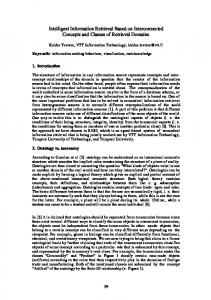
Hence, the terms in a document with the highest probability P rob1 of occurrence as predicted by such models of randomness are “non-specialty” terms. Equivalently, the terms whose probability P rob1 of occurrence conforms most to the expected probability given by the basic models of randomness are non content bearing terms. Conversely, terms with the smallest expected probability P rob1 are those which provide the informative content of the document. Figure 1.1 shows the informative content of the term “osteoporosis” within the documents of the collection WT2g of TREC-8. The term occurs in 85 documents. Notice that the term-weights decrease very rapidly when the within–document term–frequency tf diminishes.

1.5

The second component: apparent aftereffect of sampling

Now, we introduce the role played by the probability denoted by P rob2 in the fundamental Equation 1.1. The informative words are rare in the collections but, in compensation, when they occur their frequency is very high. More specifically, the 2-Poisson model captures such a duality law. There is a statistical phenomenon called by statisticians an apparent aftereffect of sampling. It may happen that a sudden repetition of success of a rare event increases our expectation of a further success to almost certainty. Laplace’s law of succession is one of the possible estimates of such an expectation. Similarly, the 2-Poisson model of IR can be explained by an aftereffect phenomenon. As already observed, all informative terms t occur to a relatively greater extent in a set


12

300

250

score

200

150

100

50

0 0

10

20

30

40

50

60

70

80

90

rank of the document

Figure 1.1: Informative content of the term “osteoporosis” with the Poisson approximation (model P ) of the Bernoulli model over TREC-8 collection.

of a few “Elite” documents. If a very rare term becomes very frequent in a document then its informative content increases very rapidly as in Figure 1.1. Let us suppose we observe in a document of the elite set of an informative word t a term-frequency tf . We saw in the last section that observing the occurrence of the term t within a given document can be abstractly studied as a success in a sequence of Bernoulli trials. Once a document d is given we have seen in the example of last Section 1.4.1 that, under certain hypotheses, we get the binomial formula for the estimate of P rob1 . (see Section 2.1.3 and Section 2.2 of Chapter 2 for a formal treatment). However, we know that if we had observed a different document then also the population would have possibly been different. Changing the population, the value of the term-frequency might well have had a different confidence interval for an accurate estimate. This happens independently from the size of the sample (the length of the document). Although we had sampled the whole document, we do not have further observations to decide whether we would have observed more occurrences of the term in the entire population of the elite set to which the document belongs. Obviously, if tf is large in the document then we take a small risk in deciding that the term tokens appeared


13

non–randomly. Small risk corresponds to a high conditional probability p(tf + 1|tf ) of having a further token of the term in the document if its length were longer than the actual one. A very small risk corresponds to a high probability, that is p(tf + 1|tf ) ∼ 1. In conclusion, the larger tf is, the closer the conditional probability p(tf + 1|tf ) is to certainty. We define P rob2 (tf ) = p(tf + 1|tf ) and 1 − P rob2 , is the risk, of accepting the informative content as a weight of the term in the document. When monetary values are involved in decisions we know that in a fair game the risk 1 − P rob2 of betting on an event is proportional to the gain. Assuming that the informative content Inf1 (tf ) of a term t in a document d is the monetary value involved in the decision of taking t as the descriptor of the document, the weight of the term in the document w turns out to be the part of the informative content Inf1 (tf ) gained with the decision of taking the term t as a descriptor of the document. In the next section we show one possible way to compute the apparent aftereffect of sampling.

1.5.1

An example of aftereffect model: Laplace’s law of succession

Once Inf1 has been computed by using a model of randomness, then the gain is computed with the conditional probability P rob2 . We will see that the so–called Laplace’s law of succession provides one interpretation of the required conditional probability. The law of succession (see Equation 3.20 at page 56) P rob2 (tf ) =

tf + A tf + A + B

can be derived with a Bayesian approach (see Sections 3.3.2 and 3.3.5 of Chapter 3). See Feller’s book [37, page 123] for a frequentist derivation of the succession law obtained with an urn model of Type II. Urns model of Type II will be discussed in Section 3.3. The relationship between frequentist and Bayesian approach expressed by De Finetti’s theorem, is presented in Sections 3, 3.1 and 3.2 of Chapter 3. B 1 Observing that 1 − P rob2 = ∝ and setting A = B = 0.5 we tf + A + B tf + A + B


14

obtain that the gain computed by Eq. (1.1) is the model P L: 

−



1  F  tf F −tf log2  p q tf + 1 tf

[model P L]

B 0.5 1 = = of the informative content. 4+1 4+1 10 Considering the example of the query on osteoporosis, the term–weighting function based

In the example of the lift the gain is only

on the gain instead of the informative content attenuates the decrease rate of the weights as can be observed in Figure 1.2. 16

14

12

score

10

8

6

4

2

0 0

10

20

30

40

50

60

70

80

90


Figure 1.2: Informative content gain (model P L) of the term “osteoporosis” over TREC8 collection.

1.6

The third component: term-frequency normalization

So far, we have introduced two probabilities: the probability P rob1 of the term given by a model of randomness and the probability P rob2 measuring the proneness of the term to appear frequently in the elite set, that is the aftereffect in sampling the term in the elite set. However, our intuition says that the magnitude of tf also depends on the document length. On the contrary, all documents are equally likely to receive tokens


15

according to the urn models of randomness. Urns do not possess a predefined volume and all documents, whether long or short, are treated equally. Briefly, the normalized term-frequency is the estimate of the expected term frequency when the document is compared with a given length (typically the average document length). We have a bivariate distribution of the number of tokens of a term and the length of documents. Once this distribution is obtained, the normalized term-frequency tf n is used in Formula 1.1 instead of the non-normalized tf . We have called the process of substituting the normalized term-frequency for the actual term-frequency the second normalization of the informative content. Despite our intuition about the dependence between frequency and length, Harter couldn’t find any general relationship between the term-frequency and the document length. Harter asserts that [52, page 23] We assume that there is no relationship between the length of a document d and the number of tokens of the term t in d. In particular, we assume that there is no tendency for long documents to contain more tokens of t than short documents. A reasonable alternative hypothesis suggests itself that the probability of a document’s receiving a token to be taken to be proportional to its length. We have run a similar experiment with a larger collection and we have arrived to a different conclusion. A positive correlation exists, and a detailed discussion about this dependence can be found in Chapter 6. We have also tested Harter’s suggestion (see Hypothesis H1 on page 107) comparing it with three other hypotheses using the Bayesian method against several test collections. The second hypothesis, that we have called H2, assumes that the relative term-frequency is not constant, as in H1, but decreasing with respect to the text length. H1 approximates H2 for large lengths (see Formula 6.7 on page 107). The third hypothesis, called H3, for term-frequency normalization uses the Dirichlet priors. This last hypothesis is a direct application of the language modelling. The probabilities of terms assigned by any language model can be applied to our framework as length normalization component (see Sections 5.5 and 6.4). In this dissertation we have used the most simple and effective language model, that is that based on Dirichlet’s priors.


16

The fourth and final hypothesis, called Z for Zipf, comes from the Pareto-Feller-Zipf’s law relating the frequency of a term in the collection, and its rank in decreasing order of magnitude of the frequency (see Sections 2.5 and 6.3). The Pareto-Feller-Zipf’s law establishes a relation between a given term-frequency and the length of the text. The problem is that the rank-frequency relation only holds when the size of the text is very large. We adopted some extra assumptions in order to apply Zipf’s law to single documents. For TREC-8 the comparison among three different models, that is the Bernoulli model only (P ), the gain function of the Bernoulli model (P L) and the gain function of the Bernoulli model under the term-frequency normalization H2 (P L2) is shown in Table 1.1. Using the query “osteoporosis”, the plot of P L2 against document rank of term– weighting is less steep than for the plots of P and P L of Figures 1.1 and 1.2, as shown in Figure 1.3. A comparison with all other models, BM 25 included, is shown in Table 7.10 on page 138. 16

14

12

score

10

8

6

4

2

0 0

10

20

30

40

50

60

70

80

90


Figure 1.3: Score distribution using the term-frequency normalization component (model P L2) over the TREC-8 collection.

Chapter 1. Theoretical Information Retrieval Models

MAP

MAP@10

Pr@5

17 Pr@10

Pr@20

Pr@R

RelRet

P L2

0.2477

0.3587

0.4880

0.4580

0.3970

0.2967

2866

PL

0.2037

0.2619

0.4160

0.3620

0.3260

0.2566

2645

P

0.0527

0.0537

0.1040

0.1100

0.0960

0.0863

1446

Table 1.1: Comparison among the basic model (P ), the gain (P L), and the term– frequency normalization model (P L2) with the TREC-8 data. The evaluation measures are defined in Appendix B.1.

1.7

The probabilistic framework

Our probabilistic framework builds the weighting formulae in three sequential steps: 1. First, a probability P rob1 is used to define a measure of informative content Inf1 in Equation 1.2. We introduce five basic models which measure Inf1 . Two basic models are approximated by two formulae each, and thus we provide seven weighting formulae: I(F ) (for Inverse term Frequency), I(n) (for Inverse document frequency where n is the document-frequency), I(ne ) (for Inverse expected document-frequency where ne is the document-frequency which is expected according to a Poisson), two approximations for the binomial distribution, D (for divergence) and P (for Poisson), and two approximations for the Bose-Einstein statistics, G (for geometric) and BE (for Bose-Einstein). 2. Then, the first normalization computes the information gain when accepting the term in the observed document as a good document descriptor. We introduce two (first) normalization formulae: L and B. The first formula derives from Laplace’s law of succession and takes into account only the statistics of the observed document d. The second formula B is obtained by a ratio of two Bernoulli processes and takes into account the elite set E of a term. 3. Finally, we resize the term frequency in the light of the length of the document. We test four hypotheses: H1 - Assuming we can represent the term-frequency within a document as a density function, we can take this to be a uniform distribution, that is the density function of the term-frequency is constant. The H1 hypothesis is a variant of the verbosity principle of Robertson [87].


18

H2 - The density function of the term-frequency is inversely proportional to the length. H3 - Dirichlet’s priors produce an expected probability for the relative termfrequency which is given by Equation 6.30 as introduced at page 117 in Section 6.4. Z - Zipf’s term-frequency normalization.

1.8

The naming of models

Models are represented by a sequence αβγ where α is one of the notations of the basic models, β is one of the two first normalization factors, and γ is either 1 , 2 3 or Z according the second normalization H1, H2, H3 or Z. For example, P B1 is the Poisson model P with the normalization factor B of 4.23 with the uniform substitution tf n for tf according to hypothesis H1, whilst BE L2 is the Bose-Einstein model BE in 2.33 with the first normalization factor L of 4.19 with the uniform substitution tf n for tf according to hypothesis H2. A summary showing all possible combinations is in Table 1.2.

1.9

The component of query expansion

In Chapter 8 we will use the same basic model of randomness used to define Inf1 to expand also the original query. In principle, the query expansion problem is less difficult than the term–weighting problem. Once a first ranking is produced by the query-document matching function, the top documents in the list are most probable members of the elite set of the query. The actual probability depends on the initial precision of the system. A set of the first few retrieved documents may be taken to be a sample of the elite set of the query. Thus we may pool the content of these document into a unique document–sample to be used in a second ranking. We do not need to normalize the frequencies in each document and the informative content Inf1 can be used directly to extract a term-weight in the elite set. The terms with the highest score can be added to the original query with a query–weight proportional to the Inf1 weight. From experiments we saw that for short queries like those submitted to the WEB search engines made up of at most three or four terms, only 3 documents and up to 10 new terms added to the query are sufficient to


19

Basic Models P

Poisson approximation of the binomial model

Formula 4.7

D

Approximation of the binomial model with the divergence

Formula 4.8

G

Geometric as limiting form of Bose-Einstein

Formula 4.10

BE

Limiting form of Bose-Einstein

Formula 4.11

I(ne )

Mixture of Poisson and inverse document-frequency

Formula 4.15

I(n)

Inverse document-frequency

Formula 4.13

I(F )

Approximation of I(ne )

Formula 4.16

First Normalization L

Laplace’s law of succession

Formula 4.18

B

Ratio of two Bernoulli processes

Formula 4.22

Second (Length) Normalization H1

Uniform distribution of the term-frequency

Formula 6.9

H2

The term-frequency density is inversely related to the length

Formula 6.10

H3

The term-frequency normalization is provided by Dirichlet’s priors

Formula 6.31

Z

The term-frequency normalization is provided by a Zipfian relation

Formula 6.29

Table 1.2: Models are made up of three components. For example BE B2 uses the limiting form BE of Bose-Einstein Formula 2.33, normalized by the incremental rate B of the Bernoulli process of Formula 4.22. The within–document term–frequency is normalized under hypothesis H2 of Formula 6.10


20

enhance significantly the performance in the second pass ranking. In the same chapter we will test 6 different basic formulae to perform query expansions, among these the Bose-Einstein statistics and the Bernoulli model. They perform similarly. The Bernoulli model of a document is this time different from that presented in Section 1.4.1. Unlike the Bernoulli model of a document presented in Section 1.4.1, where the trials were only all tokens of a term occurring in the entire collection, we regard each term in a document as a trial of an experiment. Then the whole text becomes a sequence of trials. We then observe a specific term t. A successful outcome for the term t is when t occurs in the document. Unlike the Bernoulli model of a document presented in Section 1.4.1, where the a priori probability of a success is the probability of retrieving the document, the a priori probability of a success here is the relative frequency of the term in the collection.

1.10

Experimental work

Since the three components of a model are independent, we have 7 × 2 × 4 = 56 basic models. We have also compared our models with the most effective models currently available in literature, that is the BM 25 and the language models. If we also consider the query expansion component the number of combination are 56 × 6 = 336. Considering that we have now available several big text collections (TREC ones), we could have reported at least 4, 000 runs. However, empirical science is made of trials and errors and we have continuously trialled experiments testing different hypotheses with improving fortune and using ever more effective variants of our models which for the sake of space are not reported. Therefore, with the explosion of all possible combinations we do not claim to have tested our framework extensively and exhaustively, though we have done a massive number of experiments. Nevertheless, we offer a consistent number of tables together and a discussion about our achievement.

1.11

Outline of the Thesis

Chapter 2 begins with the construction of the sample spaces for IR. This introductory chapter describes the probabilistic distributions and their limiting forms which are used


21

in many parts of the dissertation. Chapter 3 explores the estimation problem underlying the process of sampling. De Finetti’s theorem is used to show how to convert the frequentist approach into Bayesian inference and the derived estimation techniques are explored in the context of IR. Without a doubt, the problem of sampling from different populations is a central one in IR and therefore is treated extensively in this dissertation, for example in Sections 2.1 and 2.1.1, 2.1.2, 2.1.3 of Chapter 2, in many parts of Chapter 3, for example Sections 3, 3.1, 3.2, 3.3, 3.3.1, 3.3.2, 3.3.5 and 3.3.6. In the light of sampling from different populations we revisit a recent IR modelling approach, the language modelling (see Chapter 3 and Section 5.4). Chapter 4 introduces the notions of informative content and information gain of a term in a document. These two notions are related and constitute the first two components of our models. Examples of models relatively to each component are displayed and these are direct applications of the distributions studied in Chapters 2 and 3. Chapter 5 revisits the main IR models in the literature in the light of preceding chapters. We show that even language modelling approach can be exploited to assign term-frequency normalization to the models of divergence from randomness. For this reason this chapter precedes the term–frequency normalization fully developed in Chapter 6. In Chapter 7 we merge the three components and introduce the full models of randomness. Chapter 8 introduces a novel framework for the query expansion. This framework is based on the models of divergence from randomness and it can be applied to arbitrary models of IR, divergence-based, language modelling and probabilistic models included. Experiments are diluted along with all chapters, but results are summarized in the final Chapter 9 together with a discussion about open problems and new research directions.


22

Chapter 2

Probability distributions for divergence based models of IR This chapter introduces the appropriate statistical and mathematical tools to formalize several problems that we have encountered in Information Retrieval. They arise in connection with the following situations. 1. In the first chapter we have introduced the Bernoulli model of IR, in which a document was conceived as an experiment. A document is treated as a sample over a population. The outcome of an experiment is either the occurrence (success) or not (failure) of a specific term within the document. A document collection D can be thus conceived as a collection of samples over different populations. What, on these data from multiple sampling, will be the probability that a given word occur in an arbitrary document? What is the probability that a given word frequency is observed in a given document? 2. Taking a different point of view of the same problem: a term distributes F occurrences over a set of documents. What is the probability of having a particular within-document frequency configuration over the entire collection? What is the probability of observing a term-frequency tf within an arbitrary document? The basic spaces formalizing these problems will be deployed to define the basic models of Information Retrieval. Similarly, let E be a subset of the collection D. What is the probability of observ23

Chapter 2. Probability distributions for divergence based models of IR

24

ing a term-frequency FE within the subset E? The basic spaces formalizing this problem will be employed to define the models for query expansion in Information Retrieval. 3. We have a collection of documents of different lengths ld . Our intuition says that the term–frequency is related to the length of the document. What is the correlation, if any, between the within-document term-frequency tf and the length of a document? Any possible answer can be used to normalize the term–frequencies with respect to a standard document length within the basic models of Information Retrieval. 4. Let X be the random variable counting the number of words which have a frequency F in the collection. What is the distribution of X varying F ? How this number is related to the sample space size and the population of the experiment? How does the value X = F affects the observation of a term-frequency tf in a document as described in situation 3? 5. How can we model the fact that the terms which are rare events in the collection are the most informative and they become even more informative when they appear very densely in a few documents? In order to find answers to all these questions we need to define the probability spaces that we will use (see Section 2.1). Then, we introduce the basic model of randomness for IR, that is the binomial model. We derive some computational forms, the limiting forms, necessary for an effective implementation in the Information Retrieval systems. These simplified versions of the binomial law will be central in many application contexts of Information Retrieval (see Sections 2.2, 2.2.1, 2.2.2, 2.2.3 and 2.2.4). The second part of question in 2 can be also answered using the hypergeometric distribution. Using the terminology of statistics, when balls are drawn from one or more urns, while the binomial distribution assumes replacement in the hypergeometric model the extracted balls are not replaced into the urn. In practice, the hypergeometric distribution does not differ much from the binomial distribution when the sample size is very large. However, Information Retrieval deals with very small probabilities and thus the performance of the two models can be significantly different.


25

The hypergeometric distribution is useful to support the query expansion process and is the outcome of the compounding of the binomial with the Beta distribution (see Sections 2.3, 8.6 and 2.6.1). This specific compounding is introduced in connection with the language model and a particular term-frequency normalization of question 3. Another alternative model to the binomial distribution is based on Bose-Einstein statistics. The Bose-Einstein model is introduced in Sections 2.4, 2.4.1 and 2.4.2. In Bose-Einstein statistics the balls of the same colour are indistinguishable, so that many possible arrangements become indistinguishable. Finally, the fat–tailed distributions are introduced (see Section 2.5). These distributions occur when we try to classify the alternative outcomes of a sample space by their frequencies as stated by the question in 3. The most famous fat-tailed distribution in Information Retrieval is the Zipf distribution 2.5.1.

2.1

The probability space in Information Retrieval

Renyi, in his book on probability theory [85], recommends giving great attention to the construction of probability spaces, although in many applications of probability theory the probability space is implicitly assumed. In Information Retrieval we talk mainly of frequencies of terms in a collection of documents and therefore following Renyi’s suggestion, our first intention is to provide a clear definition of these entities, that is the terms and the documents, within a probability space. Information Retrieval deals with discrete probability spaces. The first notion which is defined in a probability space is the outcome of an experiment. An outcome lies into a set of mutually exclusive results. We call this set the basic space or the sample space Ω of the probability space. The algebra of events A of the probability space is made up of all subsets E ⊆ Ω. The probability distribution P is defined on the algebra of events A. The algebra of events is interpreted as the set of all observable events.


2.1.1

26

The sample space V of the terms

Cooper and Maron [22] developed a theory of indexing which they called Utility-Theoretic Indexing because it was based on utility theory. In their approach index terms are assigned to documents in such a way as to reflect the utility (or value) that the documents are expected to provide to users. Although Cooper and Maron use utilities and not probabilities, they observe that in both Probabilistic and Utility-Theoretic Indexing the fundamental conceptual construct is the event space Ω. They say:

Utility-Theoretic Indexing is related to (and if random draws are imagined to be made from it, can in fact be interpreted as) an “event space” in the statistician’s sense.

We can define several basic spaces Ω for Information Retrieval. One basic space Ω of Information Retrieval is the set V of of terms t. This set is called the vocabulary of the document collection. Since Ω = V is the set of all mutually exclusive events, Ω can also be the certain event with probability

P (V ) =

X

P (t) = 1

t∈V

The probability distribution P assigns thus probabilities to all sets of terms of the vocabulary. We would try to use this sample space directly if all probabilities P (t) were known in advance. Unfortunately, the basic problem of IR is to find an estimate for P (t). Estimates are computed on the basis of sampling and the experimental text collection furnishes the samples needed for the estimation. The main question is how we formally treat two arbitrary but heterogenous pieces of texts, for example the text of this chapter as one and an article from a sport newspaper as the other. Can they be considered as two different samples over two different populations or according to the most reductive assumption as a single sample over the same population? Indeed, the full range of different perspectives can be useful and can be successfully exploited to define query– document matching functions. The next Sections and Chapter 3 develop this idea.


2.1.2

27

Sampling with a document

Another fundamental notion which needs be defined in Information Retrieval is how we conceive a document or a collection of documents in terms of our probability space. The relationship of the document with the experiments is made by the way in which the sample space is chosen. The term experiment, or trial, is used here with a technical meaning rather than a general common sense. Thus, we can say that a document is an experiment and we mean that the document is a sequence of outcomes t ∈ V , or more simply a sample of a population. Similarly, we may talk of the event of observing a number Xt = tf of occurrences of a given word t in a sequence of experiments. In order to formally discuss this event space, however we should introduce the product of the probability spaces associated with the experiments of the sequence, but this formalism is unnecessarly pedantic. An easier way to introduce our sample space is to associate a point event with each possible configuration of the outcomes. The one-to-one correspondence defines the sample space as

Ω = V ld

where ld is the number of trials of the experiment (in this case, the length of a document). We can suppose that each outcome does or does not depend on the outcomes of the previous experiments. If the experiments are designed so that an outcome is conditioning the next outcomes then the probability space is not invariant over the sequence of trials and thus the (projection of the) probability distribution on V is different at each trial. To establish the simpler case when the probability space is invariant, in Information Retrieval, the term independence assumption is often made. Then, all possible configurations of Ω = V ld are considered equiprobable. In the case of equiprobable configurations, together with the assumption that the experiments are independent, we can consider each document a a Bernoulli process. The probability spaces of the product are invariant and the probability of a given sequence is the product of the probabilities at each trial. Therefore, if p = P (t) is the prior probability that the outcome is t and the


28

number of experiments is ld we obtain that the probability of Xt = tf is equal to: 



 ld 

P (Xt = tf |p) = 

(2.1)

tf

tf l −tf p q d

which is the sum of the probabilities of all possible configurations having tf outcomes t out of ld . P (Xt = tf |p) is a probability distribution because X

P (Xt = tf |p) = (p + q)ld = 1

t∈V

More generally, the probability distribution is the multinomial (see Equation B.11 in the Appendix) 

(2.2)

P ({tft }t∈V |{pt }t∈V ) =  



ld tf1 . . . tfV

 tf1 tf  p 1 · · · pV V

which holds in the case that we estimate the probability of an arbitrary configuration satisfying the condition (2.3)

tf1 + . . . + tfV = ld

Turning back to the binary case, that is when only a term is observed, if we estimate the probability p of occurrence, when p is unknown, then the Bayes’ theorem is used: If e1 , . . . , en are mutually exclusive events of the basic space Ω and Y ∈ {e1 , . . . , en }, then P (Y |X) =

P (Y )P (X|Y ) n X

P (ei )P (X|ei )

i=1

In our case: P (p|Xt = tf ) =

P (p)P (Xt = tf |p) n X

P (ei )P (Xt = tf |ei )

i=1

remembering e1 , . . . , en are all mutually exclusive events of the basic space; P (p|Xt = tf ) ∝ P (p)P (Xt = tf |p) The component P (X|Y ) = P (Xt = tf |p) is the likelihood of the posterior probability P (Y |X). Details and discussions about the application of Bayes’ theorem to the estimation problem in IR are all in Chapter 5. We will see that the likelihood is maximized tf . For this reason this expected frequency is also when p is the expected frequency ld


29

called the maximum likelihood. We will see also that the priors P (ei ) do not have much influence on the value of the posterior probability P (p|Xt = tf ) when the sample size, i.e. the number of trials ld , is large. The estimation problem becomes critical when the sample size is small. In this situation, subjectivity arises in the possible choice of the prior form. The subjectivism in assigning priors is somehow paradoxical, because the term prior derives from the use in logic to denote the a priori statements which are independent of experience and thus they are logically true and objective. As it was observed by Jeffreys this term has been used in so many other senses that the only disambiguation would be to abandon it [66]. However we continue to use the term while understanding that its meaning is slippery. With the choice of the prior distribution, the maximization of the likelihood may greatly diverge from the maximization of the a posteriori probability. De Finetti’s Theorem is used to explain that the estimation problem with the Bayesian approach can be seen as an alteration of the “frequentist” underlying model (see Chapter 5). Instead of drawing balls from a single urn with independent trials and a constant probability of success one can use a model with several urns, one for each trial, and with an arbitrary (not uniform) probability distribution of success. The subjectivism of the Bayesian approach then consists in deciding the most suitable initial distribution for the set of outcomes.

2.1.3

Multiple sampling: placement of terms in a document collection

We here abandon the hypothesis of having a single sample, as an homogenous piece of text as was assumed in the last Section 2.1.2, and we are going to consider that we have several samples, for example a collection D of documents. The situation of having a collection of N documents is abstractly equivalent to the scheme of placing a certain number T otF rD of V coloured types of balls in a collection of N cells. For each term t ∈ V a possible configuration of ball placement satisfies the equation (2.4)

tf1 + . . . + tfN = Ft

and the condition (2.5)

F1 + . . . + FV = T otF rD

where Ft is the number of balls of the same colour t to be distributed in the N cells.


30

We have thus implicitly changed the basic space. The outcome of our experiment will be the documents d in which the ball will be placed. Again we will have many possible configurations consistent with the number of coloured balls. The number of solutions of Equation 2.4 is again the multinomial distribution (see Equation B.11 in the Appendix), under the hypotheses that all configurations are equiprobable and exchangeable: 



(2.6)

M (Ft , {tfi }I=1,...,N , {pi }i=1,...,N ) = 

Ft



tf1 . . . tfN

 tf1 tf  p1 · · · pN N

where the priors pi is the prior probability that the document di contains the given term t. In absence of further evidence, such as the document length l, we may assume 1 the uniform distribution for pi , that is p = . Similarly, the number of solutions of N Equation 2.5 is the multinomial distribution 

(2.7)



 T otF rD  F1 F  p1 · · · p V V

M (T otF rD , {Fi }I=1,...,V , {pi }i=1,...,N ) = 

F1 . . . F V

where the priors p is the prior probability of having in a collection a term-frequency Fi . As we observe in Section 2.5 the priors may follow, for example, the Feller-Pareto law or 1 a uniform distribution with pi = . V It is easy to reduce the multinomial case to the binary case for sake of simple implementation. It can be done by assuming that the only two outcomes are the success or failure of observing the term t in a given document or in the collection. For the multinomial 2.6 the reduction is: 

(2.8)



 Ft 

B(Ft , tfi , p) = 

tfi

p

tfi Ft −tfi

q

We can further assume that all configurations which are equal under exchanges are also indistinguishable, that is all sequences which are equal under permutations must be counted as the same event. With that assumption we obtain the so called Bose-Einstein statistics (see Section 2.4). The basic sample spaces for Information Retrieval have now been introduced, and we can thus proceed to look at the main probability distributions which will be used to define the models for retrieval and query expansion.


2.2

31

Binomial distribution: limiting forms

We saw that the term independence assumption in Information Retrieval regards a document as a Bernoulli process. For example, we saw that in the binary sample case, a document is made up of a set of independent trials with a constant probability p of success, which is the probability that we encounter a specific term in a given position of the text. Indeed, Bernoulli trials are repeated and independent trials with only two possible outcomes, having constant probabilities p (success) and q (failure). Similarly, in the multiple binary sampling we derive a binomial distribution. Thus, we encounter the binomial distribution for both single and multiple sampling. Let us now treat the binomial case independently from the specific type of sampling. We would like to find useful approximations of the binomial for practical reasons. Since the outcomes of a Bernoulli process are exclusive events, the probabilities satisfy the condition: p+q =1 The probability of having k successes out of F Bernoulli trials is given by the combinatorial formula 2.8 that is





 F  k F −k p q

B(F, k, p) = 

k

B(F, k, p) is a probability distribution because 1 = (p + q)n =

F X

B(F, k, p)

k=0

We use the binomial B(F, k, p) extensively in the implementation of our retrieval models and query expansion models. Therefore a workable approximation of B(F, k, p) is necessary. The next Sections display several limiting forms of the binomial distributions.

2.2.1

The Poisson distribution

Assuming that the probability p decreases towards 0 when F increases, but λ = p · F is constant, or moderate, an approximation of Equation 2.8 is the Poisson distribution (2.9)

B(F, k, p) ∼

e−λ λk k!


32

The value λ is both the mean and the variance of the distribution. Further approximation may be obtained through the Stirling formula, which approximates the factorial number as follows [37]: (2.10)

k! =

√

2π · k k+0.5 e−tf

A refinement of Equation 2.10 is (2.11)

k! =

√

−1

2π · k k+0.5 e−tf e(12·k+1)

For example, Feller [37] shows that the approximation error for 100! with equation 2.10 is “only” 0.08%. √

B(F, k, p) ∼

(2.12)

e−λ λk 2π · k k+0.5 e−k e(12·k+1)−1

The probability in expression 2.12 does not find a direct implementation, but it is used as argument of the logarithmic function, that is: (2.13) − log2 B(F, k, p) ∼ k · log2

k λ

+ λ+

1 12·k

− k · log2 e + 0.5 · log2 (2π · k)

We will see that − log2 B is conceived as the amount of information content related to the term t, when F and tf are interpreted as the frequencies of the term in the collection and in the document respectively. The notion of information content is introduced in Section 4.2.

2.2.2

The divergence D

The fundamental Formula 2.8 of the binomial distribution can be equivalently expressed using the information theoretic divergence D [85], which is defined as: (2.14)

D(φ, p) = φ · log2

φ (1 − φ) + (1 − φ) · log2 p (1 − p)

D(φ, p) is called the divergence of φ from p. With the divergence Formula 2.8 becomes (2.15)

B (F, k, p) =

2−F ·D(φ,p)

1

(2π · k(1 − φ)) 2

1+O

1 F

where k is the number of successes, out of F Bernoulli trials, p is the constant probability k of success in each trial, φ = , O F1 is the error of the approximation. F


33

To obtain the new approximation of Formula 2.8 of the binomial distribution Renyi applied Stirling’s formula. The version of Equation 2.15 with the logarithmic is: (2.16)

− log2 B(F, k, p) ∼ F · [D(φ, p) + 0.5 log2 (2π · φ · (1 − φ))]

1 The error of the approximation with the logarithm is still O , because F

log2 1 + O

1 F

=O

1 F

This equality is obtained using the MacLaurin series (Taylor series expanded about 0) of log2 (1 + x).

2.2.3

Kullback-Leibler divergence

Let us assume the approximation of 2.15 of the binomial distribution with the information theoretic divergence of φ from p, where φ from p are defined as in Section 2.2.2. Without loss of generality we may also assume that p < φ in Formula 2.16. Indeed, we can show that in the application of the binomial distribution to both term-weighting and query expansion, the definition of p and φ will satisfy the relation p < φ. Under the assumption of p < φ, the contribution (1 − φ) log2

1−φ 1−p

negative. Also, both p an φ are very small and thus log2

in the divergence D(φ, p) is

1−φ 1−p

, which can be easily

shown to be approximately p − φ, is also close to 0. Therefore, it is straightforward to derive a further approximation of the Bernoulli process by means of the so-called asymmetric Kullback-Leibler divergence KL(φ, p): KL(φ, p) = φ · log2

(2.17)

φ p

The approximation of the binomial with the logarithm is (2.18)

− log2 B(F, k, p) ∼ F · [KL(φ, p) + 0.5 log2 (2π · φ · (1 − φ))]

The error of the divergence approximation is the same as in the previous section.

2.2.4

The X divergence

Now, we further approximate Formula ( 2.16). First, let us introduce the function g(x) = x · ln

x p


34

with 0 ≤ x, p ≤ 1. Thus, x 1 g(p) = 0, g 0 (x) = 1 + ln , g 00 (x) = p x The Taylor series of g(x) is: g(x) = g 0 (p)(x − p) + (x − p) +

=

g 00 (p) 2p (x

1 2p (x

− p)2 + O((x − p)3 )

− p)2 + O((x − p)3 )

Using the notation p1 = p, p2 = q, φ1 = φ and φ2 = 1 − φ, we can easily derive: X

g(φi ) =

P

i=1,2 (φi

− pi ) +

1 i=1,2 2pi (φi

P

− pi )2 + O((argi=1,2 max(φi − pi )3 )

i=1,2

Since X

(φi − pi ) =

P

i=1,2 φi

−

P

i=1,2 pi

=0

i=1,2

and |φ1 − p1 |3 = |φ2 − p2 |3 = |φ − p|3 we derive: (2.19)

X

g(φi ) =

i=1,2

1 X (φi − pi )2 + O(|φi − pi |3 ) 2 i=1,2 pi

Therefore, the divergence D can be approximated as: D(φ, p) = log2 e ·

X

g(φi )

i=1,2

(2.20) The function χ2 (φ, p) =

=

log2 e X (φi − pi )2 + O(|φi − pi |3 ) 2 i=1,2 pi

=

log2 e (φi − pi )2 + O(|φi − pi |3 ) 2 pq

X (φi − pi )2 i=1,2

pi

is called the χ2 divergence of φ and p. The ap-

proximation of the binomial is easily derived from Equation 2.16 by substituting D(φ, p) for the right hand side of Equation 2.20: log2 e χ(φ, p) + 0.5 log2 (2π · φ · (1 − φ)) − log2 B(F, k, p) ∼ F · 2

(2.21)


2.3

35

The hypergeometric distribution

The hypergeometric distribution plays an important role in sampling. One application of the hypergeometric distribution is shown in Section 8.6 and concerns the definition of a new model for query expansion. The hypergeometric distribution can be applied to the following problem of sampling. There is a population D of T otF rD tokens and a number F of tokens are of the same term t. A sample E of D is chosen at random. In the query expansion process E will be instead a set of relevant or pseudo–relevant documents, that is a set of documents retrieved after a first retrieval pass. In the chosen sample E we then observe a number FE of tokens of the same term t. The hypergeometric distribution defines the probability P (FE |D, E) of observing exactly FE tokens in the sample. The number of ways we can choose the tokens of the term t in the sample is 



 F 

 

FE

The number of possible ways of combining the remaining tokens in the sample is instead: 



 T otF rD − F 

 

T otF rE − FE

The total number of possible ways of combining all tokens is: 



 T otF rD  

T otF rE



Then the probability of having the sample E is thus the ratio: 





 F   T otF rD − F  

(2.22)

P (FE |D, E) =

FE



T otF rE − FE







 T otF rD  

T otF rE



The last relation can be rewritten by swapping T otF rE and F : 





 T otF rE   T otF rD − T otF rE  

P (FE |D, E) =

FE



F − FE





 T otF rD   

F




36

A limit theorem for the hypergeometric distribution (see [37, page 59]) is: 



 T otF rE  

FE

 pD −

FE T otF rD

F E

qD −

T otF rE − FE T otF rD

T otF rE −FE





 T otF rE  FE T otF rE −FE (2.23) < P (FE |D, E) <   pD q D

FE

T otF rE 1− T otF rD

0 and β > 0. U is said to have a Feller-Pareto distribution. With the Feller-Pareto distributions we are able to introduce the generalized, the classical and the standard Pareto distributions. The standard Pareto distribution is the continuous analogue of the standard discrete Zipf distribution. By definition the Feller-Pareto probability density function derives from the Beta distribution B.6[see Appendix B.1] by substituting (1 + U )−1 for Y , that is fY (y, α, β) = fU (u, α, β) =

Γ(α + β) α−1 y (1 − y)β−1 = Γ(α)Γ(β) |Y =(1+U )−1 Γ(α + β) Γ(α)Γ(β)

(2.33)

=

1 u+1

α−1

u u+1

β−1

−dY dU

α−1 β−1 Γ(α + β) 1 u − (u + 1) 2 Γ(α)Γ(β) u + 1 u+1 Γ(α + β) (u + 1)−(α+β) uβ−1 Γ(α)Γ(β) with u > 0

=

Chapter 2. Probability distributions for divergence based models of IR Equation 2.33 follows from

43

dY − = −(U +1) 2 , U being a decreasing function with respect dU

to Y .

The generalized Pareto distribution The generalized Pareto distribution of a random variable W is obtained from a linear combination of a power of U , where U is the Feller-Pareto distribution with probability density function of Equation 2.33, as follows: W (µ, σ, γ, α, β) = µ + σU γ

(2.34) If W = µ + σU γ then

U=

W −µ σ

1 γ

The probability distribution P (w) of the random variable W is thus given by the probability of the event W > w that is: W −µ P (W > w) = P (U > σ with w > µ

(2.35)

Deriving U =

W −µ σ

1 γ

)

1 γ

with respect to W we get: dU 1 = dW γσ

W −µ σ

1 −1 γ

From this derivative and Equation 2.33, we easily obtain the probability density function of the generalized Pareto distribution:

fW (w) =

Γ(α + β) Γ(α)Γ(β)

· = (2.36)

Γ(α + β) Γ(α)Γ(β)γσ

w−µ σ

w−µ σ

β−1 γ

w−µ σ

1 γσ

1 γ

!−(α+β)

1 γ

·

+1

w−µ σ

1 −1 γ

!−(α+β)

+1

with w > µ

w−µ σ

β −1 γ


44

The classical Pareto distribution The classical Pareto distribution is obtained from the generalized Pareto distribution W (σ, σ, 1, α, 1), that is with: µ = σ and γ = β = 1 The classical Pareto distribution has the probability density function fW (w) = (2.37)

Γ(α + 1) Γ(α)σ α σ

=

w σ

w σ

−(α+1)

with w > σ

−(α+1)

with w > σ

The classical Pareto distribution is then Z

P (W > x) =

xα

σ

σ

w σ

−(α+1)

−α

dw = 1 −

x σ

The discrete analogue of the classical Pareto distribution: Zipf ’s law Suppose that the random variable X takes the discrete values 0, 1, 2, . . . or 1, 2, . . . and that X has a fat-tailed distribution. Consider a sample made up of n observations. Suppose that there are V possible outcomes and that their frequency is such that p(r + 1) = P (X = r+1) ≤ p(r) = P (X = r). According to [7] Zipf distributions are discretized Pareto distributions. The discrete analogous of Formula 2.36 is defined as:

P (X ≥ r) =

(2.38)

1+

r − r0 σ

1 !−α γ

r ≥ r0

For γ = α = σ = 1 and r0 = 0 we obtain the standard Zipf distribution: P (X ≥ r) = (1 + r)−1 r ≥ 0

(2.39) Note that (2.40)

P (X = r) = P (X ≥ r) − P (X ≥ r + 1) = r−1 (1 + r)−1

For γ = 1 we obtain the Zipf distributions which are the discrete analogues of the classical Pareto distributions:

(2.41)

P (X ≥ r) =

r − r0 1+ σ

−α

r ≥ r0


45

The standard Pareto distribution The standard Pareto distribution of a random variable Z is obtained from the generalized Pareto distribution W (0, 1, 1, 1, 1). Its probability density function is: fZ (z) = (1 + z)−2 with z > 0

(2.42)

2.6

Mixing and compounding distributions

Many distributions can be constructed from different distributions by a process defined as compounding. We are using here the terminology of [67]. Let X have the the probability distribution P (X|Y ) and Y is another random variable which instead has probability distribution P rob(Y ). Then the compounding of P with P rob is Z

(2.43)

+∞

C(X) =

P (X|c · Y )dP rob(Y )

−∞

where c is a constant. Let Pi be a set of probability distributions and fi a set of values such that X

fi = 1

i

then the the mixture of the probability distributions Pi is X

(2.44)

fi Pi

i

2.6.1

Compounding the binomial with the Beta distribution

In Section 3.3.5 of Chapter 5 we compound the binomial with the Beta distribution and therefore we show here, as an example, how to compound the binomial distribution of Equation 2.8 with the Beta distribution of Equation B.6 assuming that the prior p is the parameter Y in the compounding Relation 2.43. 



 F  k F −k p q

P (X = k|p) = 

(2.45)

P rob(p) =

k

Γ(α + β) α−1 β−1 p q Γ(α)Γ(β)


46

Note that if Y = p then dP rob(p) = P rob(p)dp. Hence, the compounding is 

 1

Z

C(X = k) = 0

 F  k F −k Γ(α + β) α−1 β−1 p q dp p q 

Γ(α)Γ(β)

k

which reduces to 



Z  F  Γ(α + β) 

C(X = k) = 

Γ(α)Γ(β)

k

1

pk+α−1 q F −k+β−1 dp

0

That is 



(2.46)

 F  Γ(α + β) Γ(k + α)Γ(F − k + β) 

C(X = k) = 

Γ(α)Γ(β)

k

Γ(F + α + β)

We already know that C(X = k) is a probability distribution for De Finetti theorem (see Theorem 5). However, it is of some utility to prove it directly. In order to show that 2.46 is a probability distribution we must verify that

PF

k=0 C(X 

=  k) is equal to 1.

 x   denote the real

Let x be any real number and r be a positive integer. Let 

r

number x · (x − 1) · · · (x − r + 1) r! If a > 0 then [37, Problem 20 of Chapter II] 



 −a  r Γ(a + r)   = (−1)

r!Γ(a)

r

where Γ is the Gamma function of Equation B.1 in Appendix B.1. Relation 2.46 can be rewritten as a generalized form of the hypergeometric distribution, see Relation 2.22, with binomials containing negative real numbers: 





 −α    (−1)F −k 

(−1)k  (2.47)

k

C(X = k) =





−β F −k

 



 −(α + β)  

(−1)F 

F

From [37, Problem 9 of Chapter II]   F X  −α     k=0

k



−β F −k





  −(α + β)  = 

F


which proves that

F X

47

C(X = k) = 1

k=0

2.7

Summary and Conclusions

We have presented different probability spaces of IR: the Bernoulli model and its limiting forms, the hypergeometric distribution, Bose-Einstein statistics and its limiting forms, the compound of the binomial distribution with the beta distribution, and the fat-tailed distributions. The components of the models of divergence from randomness are based on these distributions.


48

Chapter 3

The estimation problem in IR The parameter estimation in Information Retrieval was first stated by Van Rijsbergen relatively to the probabilistic term-weighting model [118]. The interdependencies between parameter estimation and the properties of probabilistic models are also studied in [42]. Van Rijsbergen extended the Robertson and Sparck Jones weighting formula to a linear discriminant function and to a non-linear discriminant function when the terms are not assumed independent. These discriminant functions involve several parameters which need to be estimated from a small sample of relevant documents as well as from the whole collection of documents. Van Rijsbergen anticipated and recommended the use of the relevant statistical theory needed to address the estimation problem for Information Retrieval. We fully discuss and apply that proposal. We find that the content of Good’s book [44] gives an excellent combination of historical discussion and technical details for a fruitful application of the estimation rules to the problem in Information Retrieval. We have developed an understanding that Information Retrieval can be abstractly redefined by suitable models drawing balls from or distributing balls into urns. De Finetti’s Theorem and Bayes’ rule are the central relationships in this abstract reading. Their applications allow us to introduce some “subjectivism” or “arbitrariness” in the parameter estimation problem. Fortunately, Information Retrieval is an empirical science and evaluation of the newly built term–weighting models can tell us how well the different methods perform in terms of precision measures. An alternative approach to the parameter estimation is followed by Steinhaus [112]. Steinhaus minimises the loss function (p0 − p)2 where p0 is the estimate and p is the 49

Chapter 3. The estimation problem in IR

50

unknown probability of the event. This approach will be considered in Section 3.3.4

3.1

Sampling from different populations

We can imagine sampling as the experiment of drawing balls of several colours from different urns. If the ball selection uses a single urn then we would have a single population. We call the experiment of drawing from a single urn as a sampling of Type I (we use the terminology of Good [44]). We may use a “super”-population of urns, each of them having a distribution of Type I, and we may then choose one urn and perform sampling from this urn, obtaining a second type (Type II) distribution. Thus we can define infinitely many types (Type III, Type IV etc.) of sampling by iterating this construction indefinitely. The probability estimation becomes more and more complex as long as the type complexity of the sampling increases.

3.2

Type I sampling

Frequentist approach deals mainly with binary sampling of Type I. We have a single urn and after randomly selecting a ball we observe its colour and we replace it into the urn. If the ball is of the given colour then we have a success, otherwise a failure. For each ball colour t we have an expected frequency value, the mean frequency λt , which is the number of successes r divided by the total number of successes and failures in the sampling, e.g. the size n = r + s of the sample. We assume that every sequence having r successes and s failures is equiprobable. We also assume that the sequence having r successes and s failures is the outcome of repetitive drawings. Each trial is assumed to be independent from previous ones. Such sequences are called permutable or exchangeable. If the prior p is known, then the probability of having a sequence with r successes and s failures is

(3.1)

P rob(r, s|p, d) = pr (1 − p)s

The probability of having a permutable sequence with r successes and s failures can be


51

obtain by multiplying Equation 3.1 by the binomial coefficient: 



 r+s  r s  p (1 − p) 

(3.2)

r

The symbol d in 3.1 is to recall that the values r, s and p depend on the “document model” d. This notation may be used to denote other possible random variables which are observable in the given document regarded as empirical data. We may also extend Relation 3.1 considering the statistics relative to the entire collection C, and in this case we may use the notation P rob(r, s|p, . . . , d, C). If the a priori probability of drawing t is known and is equal to p, and the size of the sample tends towards very large, then the mean

r r+s

converges to p. This comes from

the theorem of large numbers: Theorem 3 (Theorem of Large Numbers) Assume that the event A has probability p. Let us carry out a sequence of identical independent experiments. Then in the first n experiments the frequency r of successes is stochastically convergent to p, that is for all ε>0 (3.3)

lim P rob (|r − p · n| > n · ε) = 0

n→∞

However, if the a priori probability p is unknown or the size of the sample is small, then the estimation of the probability p cannot be set simply to the mean value λt of the sample. In these cases, priors are parameters and Bayes’ theorem can be used to solve the problem of a Type I probability estimation. According to Bayes’ theorem, the probability of having p as prior is: P rob(r, s|p, d) · P rob(p|d) P rob(r, s|d) r p (1 − p)s · P rob(p|d) P rob(r, s|d)

P rob(p|r, s, d) = (3.4)

=

where the denominator is Z

1

P rob(r, s|p, d) · P rob(p|d)dp

P rob(r, s|d) = 0

Z

1

= 0 Z 1

(3.5)

= 0

pr (1 − p)s · P rob(p|d)dp pr (1 − p)s · dP rob(p|d)


52

and the priors satisfy the condition: Z

(3.6)

1

P rob(p|d)dp = 1 0

The probability of Equation 3.5 can be regarded as the compounding probability of the binomial with the Beta distribution that has been studied in Section 2.6.1 of Chapter 2. The estimation of the unknown prior p as given in Relation 3.4 depends on the priors of Relation 3.6. Chernoff’s bounds tell us that, when the sample is very large, the priors are less and less important in providing an estimate for p. Theorem 4 (Chernoff Bounds) Assume the same situation as Theorem 3.3. Then, for all 0 ≤ ε ≤ 1 2 pn/3

P rob (|r − p · n| > εpn) ≤ 2e−ε

(3.7)

In this case this estimate is closer and closer to the maximum likelihood λt . Therefore, the Bayesian approach would not give a very different estimate from that if we had assumed a frequentist approach or, equivalently, a Type I distribution.

3.3

Type II sampling: De Finetti’s Theorem

If we observe carefully the mathematical form of relation 3.5, then we may assert that Bayes’ Theorem has made it possible to transform a Type I sampling into a Type II distribution. Indeed, we may read the application of Bayes’ theorem as if we were sampling balls from several urns where the probability of having a frequency p has the initial distribution function P rob(p|d). More precisely, this is the content of De Finetti’s theorem: Theorem 5 (De Finetti) A sample generated by a permutable random binary sequence can always be regarded as a binomial sampling in which the a priori probability p (Type I probability) has a Type II prior distribution function P rob(p|d). In mathematical formalism De Finetti’s Theorem can be regarded as the compounding of the binomial distribution with the distribution provided by the priors as introduced in Section 2.6 of Chapter 2. As already observed, if the sample is very large, then the priors P rob(p|d) become less important and the process reduces to a Type I probability


53

distribution. In [57] there is a simple proof of this theorem which provides also an extension of the theorem to the case that the prior distribution is defined on a finite set.

3.3.1

Estimation of the probability with the posterior probability

Bayes’ theorem provides a posterior probability of p over the empirical data compounding two probability distributions of p, the likelihood and the prior distribution. We still have to solve the problems of choosing the best estimate for p. One way is to derive the most probable value of p, that is the value for p that maximizes the posterior probability. A second way is to consider the expected value of p, that is the mean of p over the posterior distribution. In other words, we can choose either the value for p that satisfies the equation dP rob(p|r, s, d) =0 dp

(3.8)

or the expectation E(p) of the random variable p with respect to the posterior probability distribution Z

1

E(p) =

p · P rob(p|r, s, d)dp =

Z

1

p · P rob(r, s|p, d)P rob(p|d)dp

0

0

These two approaches produce different results as it can be easily verified when the prior distribution is uniform. In such a case the solution of Equation 3.8 also maximises the r likelihood P rob(r, s|p, d) and therefore coincides with the maximum likelihood (see r+s Section 3.3.3), whilst the expectation E(p) of p establishes the so–called Laplace’s Law of Succession (see Section 3.3.2).

3.3.2

Bayes-Laplace estimation

Let us suppose that in the Bayes’ relation the Type II distribution function of p is uniform, that is P rob(p|d) = c where c is a constant. Equation B.7 (see Appendix) and Equation 3.4 give the Laplace’s Law of Succession. To derive it we observe that: E(p) =

1 P rob(r, s|d)

Z 0

1

p · P rob(r, s|p, d) · P rob(p|d)dp


54

1 c pr+1 (1 − p)s · dp P rob(r, s|d) 0 c Γ(r + 2)Γ(s + 1) = P rob(r, s|d) Γ(r + s + 3) c r + 1!s! = P rob(r, s|d) r + s + 2!

Z

=

(3.9)

Similarly, exploiting Equation B.7 again: P rob(r, s|d) =

R1 0

P rob(r, s|p, d) · P rob(p|d)dp = 1

Z

=c

pr (1 − p)s · dp =

0

=c

(3.10)

r!s! r + s + 1!

Both Equations 3.9 and 3.10 imply Laplace’s Law of succession: (3.11)

3.3.3

E(p) =

r+1 r+s+2

Maximum likelihood estimation

An alternative method to Bayes-Laplace is the maximum likelihood method. Relation 3.4 can be regarded as (3.12)

Posterior Probability ∝ Prior Probability · Likelihood

If the prior probability function P rob(p|d) is assumed uniform, then: (3.13)

Posterior Probability ∝ Likelihood

To obtain the posterior probability of p, the likelihood function P rob(r, s|p, d) is maximized. The maximum likelihood estimate

r r+s

is given by the solution of the first

derivative of the likelihood: (3.14)

d P rob(r, s|p, d) = pr−1 (1 − p)s−1 (r − (r + s)p) dp

d P rob(r, s|p, d) = 0. dp An algorithm for computing maximum likelihood estimates, the so-called EM algo-

r r+s

is the value for which the likelihood is maximised, that is when

rithm, from incomplete data is presented by Dempster, Laird and Rubin in 1977 [32, 79]. In situations where data are complete the maximum likelihood estimate is easy to compute. When data are incomplete some unknown parameters can be introduced to make


55

the data complete. The EM algorithm is an iterative computation of the maximum likelihood made into two steps. In the E-step the expectation of the unknown parameters Θ is computed. The M-step finds the estimates of the parameters which maximize this expectation. An application of the EM algorithm to the computation of the probability mixture parameter of the language model can be found in [59].

3.3.4

Estimation with the loss function

We apply the methodology used by Steinhaus [112] to the problem of estimation. Suppose we have a binary sample where the probability of success is p. As stated in De Finetti’s theorem, see Section 3.3, suppose we also have a prior probability distribution for p. The loss function I(x, r) is (p − x)2 where x is our estimate and p is the unknown probability p. Thus starting from Bayes’ rule 3.5 with r + s trials the loss function is: 1

Z

I(x, r) =

P rob(r, s|p, d) · P rob(p|d)(p − x)2 dp

0 1

Z

(3.15)

=

pr (1 − p)s (p − x)2 · dP rob(p|d)

0

It is easy to observe that

I(x, r) =

E(p2 − 2xp + x2 )

= E(p2 ) − 2xE(p) + x2 Therefore I(x, r) is minimised when dI(x, r) = 0 ⇔ x = E(p) dx Thus, minimising the loss function turns to be equivalent to the decision of choosing as an estimate the expected value E(p) of p as defined in Section 3.3.1.

3.3.5

Small binary samples

If the sample is not significantly large, then results obtained from Theorem 5 depend heavily on the priors and thus its use needs an estimation of the priors P rob(p|d). In such a case the maximum likelihood λt for the Type I distribution in Relation 3.1 is not very relevant. Although it may be considered for its limiting property provided


56

by the theorem of large numbers as less subjective estimate of the priors than other possible estimates. More generally the Type II distribution function can be given by a law similar to 3.1, that is by means of the Beta distribution B.7 of Appendix B.1 instead of the uniform distribution, with parameters A and B instead of r and s. (3.16)

P rob(p|d) =

pA−1 (1 − p)B−1 A−1 (1 − p)B−1 dp 0 p

R1

Since Z

(3.17)

1

pA−1 (1 − p)B−1 dp =

0

Γ(A)Γ(B) Γ(A + B)

where Γ is the Gamma function (see equation B.1 in the Appendix), then (3.18)

P rob(p|d) =

Γ(A + B) A−1 p (1 − p)B−1 · dp Γ(A)Γ(B)

The distribution 3.18 is the Beta distribution with parameters A and B. The a posteriori probability distribution which turns out from this Type II distribution, after conditionalizing on P rob(t|d), takes the same form of Relation 3.18, that is: (3.19)

P rob(p|t, d) =

Γ(A + B + r + s) r+A−1 p (1 − p)r+B−1 dp Γ(A + r)Γ(B + r)

With a similar derivation to Equation 3.11 and similarly to the derivation used in compounding the binomial with the Beta distribution in the example of Section 2.6 of Chapter 2, the expectation of p is Bayes-Laplace (3.20)

3.3.6

E(p) =

r+A r+s+A+B

Multinomial selection and Dirichlet’s priors

In this section we assume we have several urns containing balls of different colours (terms). In each urn (document) we extract l balls (tokens) and for each colour ti we observe tf successes. Thus, each document is regarded as a small sample from an unknown population. This time we observe different terms and thus we need to generalize from the binary sampling of the previous section. The generalization of the Beta distribution, the Dirichlet distribution, is used to assign the priors in the multinomial case. Priors of a Dirichlet distribution have a set of parameters A1 , . . . , An > 0, one for


57

each colour ti . (3.21)

p(p1 , . . . , pn , A1 , . . . , An ) = A=

n X

Γ(A) n −1 pA1 −1 · · · pA n Γ(A1 ) · · · Γ(An ) 1

Ai

i=1 n X

pi = 1

i=1

Ai (A − Ai ) Ai , the variance is 2 . Obviously if all parameters are equal, A A (A + 1) then the Dirichlet distribution is uniform. If there are only two parameters, A1 and A2 , The mean of pi is

then the Dirichlet distribution is that of Section 3.3.5 obtained with the Beta distribution of Formula B.6 over A1 and A2 .


58

Chapter 4

Models of IR based on divergence from randomness This Chapter defines the basic Information Retrieval models under the following alternative assumptions: 1. A document d is a sample and a document collection is a set of samples over different unknown populations. Our experiment thus consists in drawing balls from a set of urns. In other words, the occurrence of a word t at the k-th place in a document d is abstractly equivalent to the observation of a ball of colour t at the k-th trial of the experiment relative to the sample d. 2. An alternative view, but identical in mathematical properties, is having a bag of balls of different colours which need to be placed into different bins or cells (the documents). An experiment thus consists in placing T otF rD balls of different colours t into N different cells. Each cell has the property of “attracting” the balls of colour t with different probability pt . The use of one of the two types of models depends on the problem we need to formalize. The ball extraction type is more useful to formalise the apparent aftereffect in sampling (see Section 4.6) as well as to define the class of hypergeometric distributions (see Sections 2.3, 8.6 and 2.6.1), while the occupancy type is suitable, as we have seen in Section 2.4, to describe the Bose-Einstein statistics. 59

Chapter 4.


60

In the second part of the chapter the basic Information Retrieval models are normalized. We observed in the introductory Chapter (see discussion on page 11), the nonnormalized score distribution of the informative content against document rank decreases very rapidly (see Figure 1.1 on page 12). In fact, Manmatha, Rath and Feng [75] observe that, in general, the score distributions produced by good retrieval models are initially exponential and after follow a normal distribution (see Figure 1.3 on page 16). We have seen that the informative content is additive, so that when the query is made up of two or more terms the informative content of their conjunction is the sum of the single informative content-weights. The informative content, in general, assumes very large values. For example, with the query “What is a prime factor?”, while the highest value of the informative content of the term prime is 854.0 obtained with a document d1 , the highest value of the term factor is 2419.9 obtained with a different document d2 . The two terms of the query co-occur only in d1 but not in d2 . Notwithstanding the additivity property, if we had used the informative content as document score we would have obtained the document d2 as first retrieved document, but d2 is not relevant because it does not contain the term prime. Therefore the informative content—weight does not work well under the term independence assumption since the slope of the informative content is initially very steep. The role of the first normalization of the informative content is to resize suitably the informative content of a term by using only a small part of it. The part which is left as term–weight is proportional to the risk we take in choosing the term as a descriptor of the document. Risk and gain are related by the standard law of utility theory, that is gain = risk gain + loss In the previous example, the relevant document d1 positions rightly at the first place with the gain–weight. The way we compute the risk and the gain is described in Section 4.6. Before that, we introduce the notion of informative content of a term.

4.1

Basic Models

One of the most influential ideas on our our thoughts when we proposed the models of IR based on divergence from randomness is the notion of empirical or informative content

Chapter 4.


61

of a theory which comes from the book “The logic of Scientific discovery” written by Karl Popper in 1934 [83]. Popper proposed to regard the informative content of a theory as its testability. Theories may have degrees of testability. Some theories may have more potential falsifiers than other theories, and the theories with higher degree of falsifiability are also less likely to be true. For this reason Popper calls the logical probability of a theory the proportion of the complementary set of all falsifiers of the theory. In other words, the logical probability pt of a statement t is complementary to its degree of falsifiability Inf (t). Popper gives other names to the notion of informative content, such as the degree of confirmation or the degree of corroboration. He thus proposed the following mathematical relationship between logical probability and informative content Inf (t) = 1 − pt

(4.1)

The logical reasoning adopted for falsifying theories is the modus tollens: If the theory holds, then the consequent; but the consequent is not; therefore the theory is falsified. Kemeny, Good and Hamblin

1

independently suggested the definition of the degree of

confirmation as Inf (t) = − log2 pt

(4.2)

Shannon [98, 99] in his Mathematical Theory of Communication also used the logarithmic measure for measuring the information contained in a message. Base 2 for the log corresponds to the choice of the binary digit as the unit of information. Shannon’s Theory of Communication and Popper’s ideas on the nature of information have influenced a number of philosophers and scientists [18, 10, 11, 33, 62, 61, 63] who coined the term, Semantic Information Theory, to denote the studies in Logic and Philosophy on the usage of the term information, in the sense in which it is used of whatever it is that meaningful sentences and other comparable combinations of symbols convey to one who understands them. [63] 1

Popper cites Hamblin’s unpublished thesis Language and the Theory of Information of 1955 and

Good’s report on Popper’s paper in Mathematical Review, 17, page 367.

Chapter 4.


62

Conventional information theory is not concerned with the semantic aspects of communication which are irrelevant to the engineering problem of signal transmission. Semantic Information Theory investigates the axiomatization of logical principles for assigning probabilities to sentences, and it studies the relationship between informative content and probability. Willis and Solomonoff [124, 108] use Equation ( 4.2) as a measure of the amount of information carried by an event and Goldman [43] develops information theory starting from Equation ( 4.2). A second influence on our work is the notion of randomness as it is conceived in the notion of Kolmogorov complexity [71]. Kolmogorov complexity provides a definition of a random (finite or infinite) sequence. Regular sequences can be easily compressed, while random sequences do not possess shorter descriptions. The key theorem of Kolmogorov complexity is the existence of a universal Turing machine U which computes all and only all partial recursive prefix functions. A prefix function is able to encode arbitrary sequences of natural integers using prefix-codes. An example of prefix code is the δ–code used for example to compress inverted files of Information Retrieval[126]. We saw that in a Bernoulli process if the number of trials increases indefinitely, then the maximum likelihood approaches the prior probability of success. For short sequences the priors are too conclusive that we cannot perform an “objective” or “justified” probabilistic inference. In case that we have small empirical data Solomonoff[106, 107] proposed to assign a universal prior probability p which satisfies the following Coding Theorem − log2 p(x) = − log2

(4.3)

X

2−l(p) = K(x)

U (p)=x

The equality holds up to an additive constant. 2−K(x) is the probability of having a prefix of complexity K(x), that is the length l(p) of the minimal prefix string p such that the string x is the output of the universal prefix machine U on p. The probability 2−K(x) thus represents the cost of encoding the string x by the shortest program p;

P

U (p)=x 2

−l(p)

can be reduced to the computation of the probability of

this representative up to some constant which does not depend on the string x. Random sequences thus have a large algorithmic complexity K(x) and, complementarily, a

Chapter 4.


63

smaller prior probability p(x). Thus the Coding Theorem states a powerful and theoretically appealing fact. Inductive inference can be solved using the algorithmic complexity K. For example in our framework, we may assign in principle the universal prior probability distribution to our Bernoulli trials. In practice, we have to specify an encoding language to represent our problem, which should be chosen to be as “optimal” as possible in relation to its compressibility power, and then we try to compute the encoding cost according to the chosen representation language. We may define, for example, the probability relative to the encoding cost of a binary Bernoulli process of l trials, to be the number of possible consistent configurations out of all configurations (as defined by Equation 2.3 or Equation 2.4). Therefore, the most informative sequences are those with the highest encoding cost, that is those sequences with the smallest binomial probability B(l, tf, p) (as defined by Equation 2.1 or Equation 2.8). Now, we saw that B(l, tf, p) is maximised when p is the maximum likelihood is equivalent to the fact that the divergence D of

tf l

tf l .

This

from p, as defined by Equation 2.14

of Section 2.2.2, is minimised. In case that B(l, tf, p) is minimised, we observe that the frequencies in the sample diverge from those we would get by choosing a sample at random. In other words, the successful trials do not occur in the number predicted by the Bernoulli distribution. We here mean by “random” that the trials of the sample follow a Bernoulli process. This notion of randomness differs from the notion of randomness given in algorithmic complexity theory, which is similar to Popper’s notion of objective disorder or irregularity. In our case, by contrast a random selection of the sample brings about the regularity in the frequencies anticipated by the priors. Nevertheless, the way we compute the informative content is the same, that is

− log2 pt

where the probability pt is given by different probabilistic models of the sample space.

Chapter 4.

4.2


64

The informative content Inf1 in the basic probabilistic models

In this section we assume that for each pair of a term and document, the following four random variables are given: 1. the total number of term tokens T otF rD in the collection D; 2. the term-frequency Ft in the collection; 3. the cardinality N of the collection; 4. the term-frequency tf in the document d; Let P rob1 be a probability distribution over the sample space, and let X be the random variable counting the occurrences of the term in the documents. With P rob1 (tf |Ft , T otF rD , N ) we denote the probability that X = tf with respect to the empirical data. Definition 6

The informative content of a term t in a document d is Inf1 (tf |Ft , T otF rD , N ) = − log P rob1 (tf |Ft , T otF rD , N )

In the rest of this chapter the shorter expressions Inf1 (tf ) and P rob1 (tf ) will denote Inf1 (tf |Ft , T otF rD , N ) and P rob1 (tf |Ft , T otF rD , N ). Our objective is the definition of the sample space over this population together with the assignment of a suitable probability distribution P rob1 .

4.3

The basic binomial model

We make the assumption that the Ft tokens of a non–informative word t distribute over N documents according to the binomial law. The situation is abstractly equivalent to having a sequence of F trials with N possible outcomes, the documents, at each trial. The prior probability of having a given document as outcome is p=

1 N

Chapter 4.


65

We are now interested to determine the probability of observing tf occurrences of t in a document rather than the probability of the given configuration tf1 + . . . + tfN = Ft which we have already encountered in Section 2.1.3 (see Equation 2.4). The probability of observing tf occurrences in an arbitrary document out of F Bernoulli trials is thus given by Equation 2.8, that is 



 F  tf F −tf p q

(4.4)P rob1 (tf ) = B (N, F, tf ) = 

where p =

tf

1 N −1 and q = N N

The maximum likelihood frequency of the term in the collection is (4.5)

λ=

F N

tf + 1 (see the Bayes-Laplace relation 3.11) F +2 Equation 4.4 was used by Harter to define his 2-Poisson model[52].

while the expectation E(p) of p is

We saw in Section 2.1.3 that the configuration problem can also be seen as a scheme for placing a number T otF rD of V terms in a collection of N documents. For each term t ∈ V a possible configuration of term placements satisfies Condition 2.4 and all terms satisfy the further condition (see Equation 2.5) F1 + . . . + FV = T otF rD So, the probability of a possible configuration that is consistent with the empirical data is the product of two multinomial distributions (see Equation 2.6 and 2.7), each deriving from the conditions 2.4 and 2.5. The informative content of t in a document d is thus given by 

(4.6)





 F 

Inf1 (tf ) = − log2 

tf

tf F −tf  p q 

with p =

1 N

The reader may notice that the document-frequency n (the number of different documents containing the term) is not used in this model.

Chapter 4.

4.3.1


66

The model P

The informative content 4.6 can be approximated using the Poisson distribution. We may use this approximation when the mean p · F of the Poisson distribution, which is the maximum likelihood λ of 4.5, is small or moderate in magnitude. Therefore, we assume that the number F of occurrences of the term is smaller than the number N of documents in the collection. The informative content is that defined by the estimate 2.13. This formula generates the basic probabilistic model P . The acronym P stands for Poisson. tf 1 Inf1 (tf ) = tf · log2 + λ+ − tf · log2 e + 0.5 · log2 (2π · tf ) [ model P ] λ 12 · tf F with λ = (4.7) and F N N

4.3.2

The model D

We have approximated the binomial distribution using the information theoretic divergence D and Stirling’s formula in Section 2.2.2. From Equations 2.15 and 2.14 we derive the basic probabilistic model D. The acronym 1 tf from p = . D stands for Divergence of the mean φ = F N (4.8)

Inf1 (tf ) = F · (D(φ, p) + 0.5 log2 (2π · φ · (1 − φ))) [ model D] tf 1 with φ = and p = F N

We will see that the models P and D do not produce different experimental results, so they are experimentally indistinguishable.

4.4

The basic Bose-Einstein model

In Section 2.4 we have seen that the Bose-Einstein statistics differs from the binomial distribution because all configurations satisfying Equation 2.4 are indistinguishable. The informative content Inf1 derives from the probability in Equation 2.28 (4.9)

4.4.1

Inf1 (tf ) = − log2

(N + F − tf − 2)!F !(N − 1)! (F − tf )!(N − 2)!(N + F − 1)!

The model G

In Section 2.4.1 we have approximated Equation 2.28 with the geometric distribution.

Chapter 4.


67

From Equation 2.31 we derive the basic probabilistic model G

(4.10)

Inf1 (tf ) = log2 (1 + λ) + tf · log2 1 + with λ =

1 λ

[ model G]

F and F N N

The symbol G stands for the geometric distribution. This approximation was obtained with N large, that is with F N .

4.4.2

The model BE

The second approximation of the Bose-Einstein statistics comes from a direct application of the Stirling formula (see Equation 2.33): Inf1 (tf ) = − log2 (N − 1) − log2 (e) + f (N + F − 1, N + F − k − 2) − f (F, F − k) n (4.11) f (n, m) = (m + 0.5) · log2 + (n − m) · log2 n and F N [ model BE ] m We will see that the models G and BE do not produce different experimental results, so they in practice coincide.

4.5

The tf-idf model

Let us choose a different sample space from binomial and Bose-Einstein statistics. We assign to each possible term-frequency tf in a document d the probability ptf q of the geometric distribution, where p is the prior probability that t occurs in the document. In fact the probability P rob1 (tf > 0) =

∞ X tf =1

q·p

tf

=q·p

∞ X tf =0

p

tf

1 − lim ptf +1 =q·p

n→∞

1−p

=p

Therefore, the tf-idf probabilistic model is a generalization of the model G defined in Section 4.4.1. The tf-idf model coincides with G in the case that the prior p is set equal λ F to with λ = . 1+λ N An alternative way to assign the prior p exploits the document-frequency nt , that is the number of documents of the collection containing the term t. The probability p is the nt relative document-frequency . Substituting these priors in the geometric distribution N

Chapter 4.


68

we obtain inf1 (tf ) = log2

N N + tf · log2 N − nt nt

Since in general nt N , we can assume N ∼ N − nt that is inf1 (tf ) = tf · log2

N nt

We saw that if the prior is given by the Bayes-Laplace estimate then inf1 (tf ) = tf · log2

N +2 nt + 1

We also saw that, if the prior is assumed to be of the beta form with parameters A and B, see Equation 3.20, then the Bayes rule generates inf1 (tf ) = tf · log2

(4.12)

4.5.1

N +A+B nt + A

The model I(n)

From Equation 4.12 we can generate a class of models by varying the parameters A and B. In the INQUERY Information retrieval system [2] the parameter values A and B are set to 0.5. In the absence of evidence, that is when the collection is empty with N = nt = 0, for A = B = 0.5 the a posteriori probability p has the maximum uncertainty value 0.5. We also set the values of A and B to 0.5. The basic probabilistic model I(n) is thus defined as (4.13)

inf1 (tf ) = tf · log2

N +1 nt + 0.5

[model I(n)]

The symbol I(n) stands for “model with the Inverse of the document-frequency n”.

4.5.2

The model I(ne )

As in the previous section, we derive the equation similar to that 4.12 using the prior ne + A p = , where ne is the number of expected documents containing the term N +A+B according to the binomial law 2.8. It is easy to compute this estimate from the binomial 2.8. (4.14)

ne = N · (1 − B(Ft , 0, p)) = N · 1 − q Ft

Chapter 4.


69

A new basic probabilistic model I(ne ) is thus defined inf1 (tf ) = tf · log2

(4.15)

N +1 ne + 0.5

[model I(ne )]

The name I(ne ) stands for “model with the Inverse of the expected document-frequency ne ”.

4.5.3

The model I(F ) F

Note that 1 − B(N, F, 0) ∼ 1 − e− N by the Poisson approximation of the binomial, F

and that 1 − e− N ∼ assuming that

F N

F N

with an error of order O(

F N

2

). Using this approximation and

is small, another basic probabilistic model I(F ) is thus derived from

the model I(ne ) (see Formula 4.15) (4.16)

inf1 (tf ) = tf · log2

N +1 F + 0.5

[model I(F )]

The name I(F ) stands for “model with the Inverse of the term-frequency F ”. A generalization of the I(F ) was given by Kwok [68] with the ICTF Weights (ICTF stands for the Inverse Collection Term Frequency Weights), in the context of the standard probabilistic model using relevance feedback information [90]. Kwok reported that the ICTF performed much better than Salton’s inverse document-frequency model[94]. We show that in our experiments I(F ) and I(ne ) behave similarly and irrespective to the other normalization components.

4.6

First normalization of the informative content

Starting with this section we resume the systematic exposition of the second component of the retrieval models introduced in Chapter 1. We have abstractly reproduced the Information Retrieval process as we had coloured balls to place in or extract from urns. If sampling is with replacement, then the population is not changed and the probability of extracting the same ball in a successive trial is invariant. The conditional probability of having a sequence, for example, of {red, red} when the first trial is red is the same as the prior probability of having {red}. In a Bernoulli process the “holding time” between the appearance of two balls of the same colour does not depend on how long the ball has not appeared in the past. This

Chapter 4.


70

situation is described by a process with a complete lack of memory, that is past outcomes do not modify the expectation of the event. A different situation is when we are searching for tokens of a term and after a long unsuccessful search we find a few of then in a portion of a document. It is quite likely that we have finally reached a document for which we can expect an increased rate of success in continuing our search. The more occurrences we find the higher is our expectation. We assume that this expectation is measured by P rob2 (tf ) in Formula 1.1. The probability P rob2 (tf ) has been called by statisticians an apparent aftereffect of future sampling [37, pp118-125]. The intuition underlying the aftereffect in IR is that the greater the term-frequency tf of a term in a document, the more the term is contributing to discriminating that document. There are several models for modelling the aftereffect, one of these is the law of succession of Laplace [44] discussed in Section 3.3.2. Simulating aftereffect with our urn model consists in replace the extracted ball with other balls of the same or different colour. A second possibility is to use different urns having a prior probability of being selected, but once the urn has been selected the balls continue to be drawn from the chosen urn. Feller[37, page 119] pictures the urn models of aftereffect as the results of a superhuman game of chance. If at each trial the chance of a rare event, like the occurrence of an accident, remains constant in time as expected then the population of the urn continues to be the same. But we may assume that an occurrence of that rare event has an aftereffect in the fact that it increases rapidly the chance to occur soon again. The more the rare event is observed at regular time intervals the more the chance of new occurrences of this event increases. In other words, the probability of the event in the successive interval of time is conditioned by its frequency tf in previous intervals of time. Turning back to the IR context, if tf is large then the probability that the term may select a relevant document is high. The fact that tf is large depends also on the length of the document. Moreover, relevant documents may have different lengths and we cannot predict the length of a relevant document. Therefore we assume for the moment that the

Chapter 4.


71

length of a relevant document is of arbitrary and large in size. In Section 6.2 we show how to normalize the actual document length l to a standard length. When enlarging the actual size of a relevant document to an arbitrary large size, the chance of encountering a new token of the observed term increases in accordance with the size tf of already observed tokens. We thus assume that the probability that the observed term contributes to the selection of a relevant document is high, if the probability of encountering one more token of the same term in a relevant document is similarly high. We reason that a high expectation of encountering one more occurrence will be due to some underlying semantic cause and will not be simply random. The probability of a further success in encountering a term is thus a conditional probability which approaches 1 as tf increases and becomes large. On the other hand, if successes were brought about by pure chance, then the conditional probability would tend to approach 0 as tf increases and becomes large. We need however, a method to estimate our conditional probability. We assume that the probability P rob2 (tf ) is related only to the “elite set” of the term, which is defined to be the set Et of all documents containing the term. We also assume that the probability P rob2 (tf ) in Formula 1.1 is obtained by a conditional probability p(tf + 1|tf, d) of having one more occurrence of t in the document d and that p(tf + 1|tf, d) is obtained from an aftereffect model. This probability is computed in the next two Sections.

4.6.1

The first normalization L

The first model of P rob2 (tf ) is given by Laplace’s law of succession. The law of succession in this context is used when we have no “advance knowledge” of how many tokens of a term should occur in a relevant document of arbitrary large size. The Laplace model of aftereffect is explained by Feller [37]. Feller shows that the probability p(tf + 1|tf, d) is close to

tf +1 tf +2

and does not depend on the document length.

Laplace’s law of succession is thus obtained by assuming that: i) the probability P rob2 (tf ) modelling the aftereffect in the elite set in Formula 1.1 is given by the conditional probability of having one more token of the term in the document, that is passing from tf observed occurrences to tf + 1, and

Chapter 4.


72

ii) the length of a document is very large. A Bayesian derivation of Laplace’s law of succession was given in Section 3.3.5 with Formula 3.20 at page 3.20. According to this formula we would have (4.17)

P rob2 (tf ) =

tf + A tf + A + B

Similarly, if tf ≥ 1 then P rob2 (tf ) can be given by the conditional probability of having tf occurrences assuming that tf − 1 have been observed. If A = B = 0.5 we get the following Equation (4.18)

P rob2 (tf ) =

tf + 0.5 tf + 1

Equations 1.1 and 4.18 give the normalization L: weight(t, d) = (4.19)

∝

B · Inf1 (tf ) tf + A + B 1 · Inf1 (tf ) tf + 1

The constant B = 0.5 is ignored being independent from the term and thus not influential to the ranking. In our experiments, which we do not report here for sake of space, the parameters A = B = 0.5 of Relation 4.17 performs better than other values, therefore we refer to the Formula 4.19 as First Normalization L of the informative content.

4.6.2

The first normalization B

The second model of P rob2 (tf ) is slightly more complex than that given by Relation 4.18. The conditional probability of Laplace’s law directly computes the aftereffect on future sampling. The hypothesis about aftereffect is that any newly encountered token of a term in a document is not obtained by accident. If we admit that randomness is not the cause of encountering new tokens then the probability of encountering a new token must increase (or decrease) with respect to the probability which is expected by randomness. Hence, the aftereffect on the future sampling is obtained by a process in which the probability of obtaining a newly encountered token is inversely related to that which would be obtained by accident. In other words, the aftereffect of sampling from the elite set yields a distribution which departs from one of the “ideal” schemes of randomness we described before. Therefore, we can model the aftereffect process by Bernoulli.

Chapter 4.


73

However, a sequence of Bernoulli trials is a process characterized by a complete lack of memory (lack of aftereffect). It is known that previous successes or failures do not influence successive outcomes. The lack of memory does not allow us to use Bernoulli trials, as for example in the ideal urn model defined by Laplace, since the conditional probability p(tf + 1|tf, d) would be constant for all tf . To obtain the estimate P rob2 with Bernoulli trials we use the following urn model. We add a new token of the term to the collection, having thus F + 1 tokens instead of 1 F . We then compute the probability B F + 1, tf + 1, that this new token falls into n the observed document, thus having a within–document term–frequency tf + 1 instead tf . 1 The probability B F + 1, tf + 1, is thus that of obtaining by accident one more n token of the term t in the document d out of all n documents in which t occurs when a

new token is added to the elite set. The comparison

1 n

B F + 1, tf + 1,

B F, tf,

1 n

1 1 of the new probability B F + 1, tf + 1, to the previous one B F, tf, tells us n n whether the probability of encountering a new occurrence is increased or diminished by

sampling from our urn model. ∆B of term-occurrence B in the elite set rather than of probability P rob2 of term-occurrence in the elite set. Therefore, we may talk in this case of an incremental rate

We suppose that the incremental rate of occurrence is

(4.20)

∆B = B

B F, tf,

1 n

− B F + 1, tf + 1, 1 B F, tf, n

1 n

= 1−

If the ratio of two Bernoulli processes

(4.21)

B F, tf,

1 n

B F + 1, tf + 1,

B F, tf,

1 n

1 n

B F + 1, tf + 1,

1 n

Chapter 4.


74

is smaller than 1, then the probability of having received at random the newly added token increases. Since the binomial decreases very rapidly at increasing values of the term-frequency, the larger the tf the less accidental one more occurrence of the term is. Therefore, accepting the term as a descriptor of a potentially relevant document is less risky. Equation 4.21 is a ratio of two binomials as given by Equation 4.4 (but using the elite set with p =

1 n

instead of p =

1 N ):

∆B = 1− B

(4.22)

1 n

B F + 1, tf + 1,

1 B F, tf, n F +1 =1− n · (tf + 1)

=

The equations 1.1 and 4.22 give

1 n

B F +1,tf +1,

(4.23)

weight(t, d) =

B

4.7

1 F,tf, n

· Inf1 (tf ) =

F +1 · Inf1 (tf ) n · (tf + 1)

Relating the aftereffect probability P rob2 to Inf1

In this section we set out a formal derivation of Formula 1.1, which describes the relationship between the elite set and the statistics of the whole collection, which involves showing how the probabilities P rob2 and P rob1 are combined. The use of the gain as term-weighting is completely new, as well as its relation to the apparent aftereffect of sampling. We stress that also the idea of using Inf1 for defining basic Information Retrieval models is original, although we saw that the standard tf–idf term-weighting can be interpreted as informative content (see the model I(n)). Let us assume that a term t belongs to a query q. We assume that if the term t also occurs in a document then we accept it as a descriptor for a potentially relevant document (relevant to the query q). A gain and a loss are thus achieved by accepting the query term t as a descriptor of a potentially relevant document. The gain is the amount of information we will get if the document turns out to be actually relevant. The gain is thus a fraction of Inf1 (tf ). What remains of Inf1 (tf ) is the loss, and the loss is produced in the case that the document turns out not to be relevant. This translates

Chapter 4.


75

into the equation: (4.24)

gain + loss = Inf1 (tf )

We weight the term by computing only the expected gain, namely weight(t, d) = gain The conditional probability P rob2 (tf ) of occurrence of the term t is related to the odds in the standard way (the higher its probability the smaller the gain): (4.25)

P rob2 (tf ) =

loss gain + loss

From Equation 4.25 the loss is loss = P rob2 (tf ) · Inf1 (tf )

(4.26)

For scoring documents we use only the gain, which from 4.24 and 4.26 is Inf1 (tf ) − loss

weight(t, d) = gain =

= (1 − P rob2 (tf )) · Inf1 (tf )

(4.27)

Example 1 As an example, let us consider the term “progress” which occurs 22, 789 times in a collection containing 567,529 documents. Let us use the Poisson model P for computing the amount of information Inf1 and use Laplace’s law of succession to compute the loss and the gain of accepting the term as a descriptor for a potentially relevant document. We distinguish two cases: the term-frequency in the document is equal to 0 or not. In the second case suppose tf = 11 as an example. We construct the following contingency table: Accept (tf = 11)

Not accept (tf = 0)

d is relevant

gain1 = 6.9390

loss0 = 0.04015

d is not relevant

loss1 = 69.3904

gain0 = 0

Inf1 = 76.3295

Inf0 = 0.04015

First we compute the amount of information Inf1 = 76.3295 as given by the formula 2.9 with tf = 11 and 1 − P rob2 (tf ) = 1 −

10 11

= 0.0909 from 4.18, then gain1 is obtained

by multiplying these two values. Similarly, loss1 = 0.9090 · 76.3295 = 69.3904.

Chapter 4.


76

When tf = 0 we reject the term, that is the term is considered not to be a descriptor of a potentially relevant document, so by rejecting the term we have a gain when the term “progress” is not important for predicting the relevance of the document. According to Laplace’s law of succession the gain is 0, while the loss is very small.

4.8

First Normalized Models of Divergence from Randomness

The first normalization factor of Inf1 (tf ) of Equation 4.19 is denoted by L (for Laplace), while the normalization of Equation 4.23 is denoted by B (for Binomial). First Normalized Models of IR are obtained from the basic models - P of Equation 4.7 on page 66; - D of Equation 4.8 on page 66; - G of Equation 4.10 on page 67; - BE of Equation 4.11 on page 67; - I(n) of Equation 4.13 on page 68; - I(ne ) of Equation 4.15 on page 69; - I(F ) of Equation 4.16 on page 69 applying the first normalization - L of Equation 4.19 on page 72 or - B of Equation 4.23 on page 74. For the sake of completeness we here list the 14 first normalized models of divergence from randomness which we test in this dissertation.

4.8.1

Model P L

1 tf 1 tf · log2 + λ+ − tf · log2 e + 0.5 · log2 (2π · tf ) w(tf ) = tf + 1 λ 12 · tf F (4.28) with λ = and F N N

[ model P L]

Chapter 4.

4.8.2


Model P B tf 1 F +1 tf · log2 + λ+ − tf · log2 e + 0.5 · log2 (2π · tf ) n · (tf + 1) λ 12 · tf F with λ = (4.29) and F N N

w(tf ) =

4.8.3

1 (F · (D(φ, p) + 0.5 log2 (2π · φ · (1 − φ)))) tf + 1 tf 1 with φ = , D as in Equation 2.14 and p = F N

[ model P B]

[ model DL]

F +1 (F · (D(φ, p) + 0.5 log2 (2π · φ · (1 − φ)))) [ model DB] n · (tf + 1) tf 1 with φ = , D as in Equation 2.14 and p = F N

Model GL 1 1 F · log2 (1 + λ) + tf · log2 1 + tf + 1 λ F and F N with λ = N

(4.32) w(tf ) =

4.8.6

Model DB

(4.31)w(tf ) =

4.8.5

Model DL

(4.30) w(tf ) =

4.8.4

77

[ model GL]

Model GB F +1 1 log2 (1 + λ) + tf · log2 1 + n · (tf + 1) λ F with λ = and F N N

(4.33)

w(tf ) =

4.8.7

Model BE L

[ model GB]

1 (− log2 (N − 1) − log2 (e) + f (N + F − 1, N + F − k − 2) − f (F, F − k)) tf + 1 (4.34) with f as in Relation 4.11 and F N [ model BE L]

w(tf ) =

Chapter 4.

4.8.8 w(tf ) =

4.8.9


Model BE B F +1 (− log2 (N − 1) − log2 (e) + f (N + F − 1, N + F − k − 2) − f (F, F − k)) n · (tf + 1) (4.35) with f as in Relation 4.11 and F N [ model BE B]

Model I(n)L N +1 1 tf · log2 tf + 1 nt + 0.5

(4.36)

4.8.10

w(tf ) =

[model I(n)L]

Model I(n)B F +1 N +1 tf · log2 n · (tf + 1) nt + 0.5

(4.37)

w(tf ) =

4.8.11

The model I(ne )L

(4.38)

w(tf ) =

1 N +1 tf · log2 tf + 1 ne + 0.5

[model I(n)L]

[model I(ne )L]

where ne is as in equation 4.14.

4.8.12

The model I(ne )B F +1 N +1 tf · log2 n · (tf + 1) ne + 0.5

(4.39)

w(tf ) =

[model I(ne )B]

where ne is as in equation 4.14.

4.8.13

Model I(F )L 1 N +1 tf · log2 tf + 1 F + 0.5

(4.40)

4.8.14

w(tf ) =

[model I(F )L]

Model I(F )B N +1 F +1 tf · log2 n · (tf + 1) F + 0.5

(4.41)

78

w(tf ) =

[model I(F )B]

Chapter 5

Related IR models Before we develop the last component of the probabilistic Information Retrieval models based on divergence from randomness, it is useful and important to examine the existing models for Information Retrieval, that have influenced our work. By models we include both weighting functions for document retrieval and term-indexing. A complete and detailed presentation of the probabilistic models can be found in [41, 24]. Therefore, we here do not try to survey all of them but to introduce and discuss the most important aspects of them to make a tight comparison with our work and we try and we take a technical view of them as close as possible to that used in our investigation. In particular the language modelling, described in Sections 5.4 and 5.5, are also applied to the models of divergence from randomness in Chapter 6.

5.1

The vector space model of IR

The vector space model is a class of models rather than a single model. Many models can be traced back to that implemented by the well known, the SMART system[93, 96], one of the first experimental systems of Information Retrieval. The basic matching function between the document d and the query q is obtained by considering both queries and documents as vectors d, q ∈ RV and computing the similarity of documents and queries with the cosine function of the corresponding vectors. RV is the product space of the vocabulary V . The cosine is the inner product normalized by the norms of the vectors: (5.1)

sim(q, d) = 79

(d, q) kdkkqk

Chapter 5. Related IR models

80

The term-weights making up the document vector d = (w1 , w2 , . . . , wV ) define a variant of the vector space model. The simplest term-weighting function is [96, see Chapter 3] the Inverse Document Frequency Weight

(5.2)

wk = tf log2

N +1 nt

nt is the relative document frequency of the k-th term t , that is the ratio of the N number nt of documents in which the term occurs and the number N of documents in where

the collection, and kdk =

sX

wk2 is the norm.

tk ∈d

When the within–document term-frequencies tf , relative to the terms of the query, are all the same in two or more documents, the longest document receives the smallest similarity score, since its norm kdk is larger. In the vector space model there is thus an implicit normalization of the term-frequency with respect to the document length. This problem in Information Retrieval is called length normalization. For many years the length normalization performed by the similarity induced by the cosine function in the vector space model has been considered very robust. But, on the other hand, the cosine normalization requires the computation of the norm of the documents which can be heavy in implementation. A retrieval model in order to be a genuine alternative to the vector space model must use a different method from the cosine function for normalizing the term-frequency tf . For example, it could consider the document length ld as an explicit random variable of the probability space. This is what the BM 25 formula does: the BM 25 abandons the normalization provided by the cosine for the inclusion of the document length in the weighting formula. We discuss more extensively the length normalization problem in Chapter 6.

5.2

The standard probabilistic model of IR

Information Retrieval models, vector space model included, are based on probability theory [90, 51, 119, 91, 40, 127, 117, 115, 25, 128, 82], but the meaning of the term “probabilistic” pertains to the explicit usage of relevance as an element rel of the algebra of events. In other words, a probabilistic model ranks documents satisfying the so called “Probability Ranking Principle” (P RP ) [89]. The P RP asserts that documents should be ranked according to the decreasing ordering established by the probability of relevance


81

p(rel, d|q) with respect to a given query q. Bayes’ theorem relates the a posteriori probability p(rel, d|q) with the likelihood (also called the a priori probability) p(q, d|rel) and the priors p(rel), p(t). First, term independence assumption simplifies the computation of the likelihood p(q, d|rel) =

Y

p(t, d|rel)

t∈q

where p(t, d|rel) =

   p(t|rel)

0

 

if t ∈ d otherwise

Then, Bayes’ theorem is (5.3)

p(rel, d|t) =

p(t, d|rel) · p(rel) p(t)

In the binary independence indexing model of Maron–Kuhns and Fuhr [78, 40] Bayes’s theorem is applied with a different reading, that is (5.4)

p(rel|t, d) =

p(t|rel, d) · p(rel|d) p(t|d)

All terms in the observed document d of Equation 5.4 are regarded as items of evidence in Bayes’ rule. This is equivalent to assuming that we are mainly sampling from a single document, like the sampling in the language model shown in Chapter 3. As a consequence the prior p(rel|d) should be assigned considering the document d as an item of evidence, whilst Equation 5.3 provides a prior probability to relevance which is not conditioned by the observed document. This view is actually implemented by the standard probabilistic model. Notwithstanding this discrepancy, it comes out indeed that the results are practically the same for both formalizations and we may equally draw the same final weighting formula. For the above considerations, we prefer to assume Formula 5.3 as generating formula of the standard probabilistic model. In the Croft and Harper model [27] the prior p(t) can be regarded as an approximation of the probability of occurrence of the term t in only non-relevant documents p(t|rel). This assumption leads to the relation p(rel, d|t) =

p(t, d|rel) · p(rel) p(t|rel)


82

Since p(rel) is a constant and observing that the Boolean event “t, d” in Equation 5.3 stands for t ∈ d, then we derive the posterior probability distribution of relevance: Y p(t|rel)

p(rel, d|q) ∝

(5.5)

t∈q∩d

p(t|rel)

The Robertson Sparck–Jones[90] model uses instead the cross product ratio: p(rel, d|q) ∝

(5.6)

Y p(t|rel) · p(t|rel) t∈q∩d

p(t|rel) · p(t|rel)

If the probabilities involved in relation 5.6 are estimated by using the counting measure over the set of documents and if R, r and n respectively denote the cardinalities of the set of relevant documents, the set of relevant documents in which the term t occurs and the set of documents in which the term t occurs, then we obtain (see the contingency Table 5.1): Table 5.1: The contingency table in the probabilistic model. t

t

rel

r

R−r

R

rel

n−r

N −n−R+r

N-R

n

N −n

N

Y r · (N − R − n + r)

p(rel, d|q) ∝

(5.7)

(n − r) · (R − r)

t∈q∩d

We can transform this probability into an additive weighting formula using the monotonic function log: (5.8)

p(rel, d|q) ∝

X

log

t∈q∩d

r · (N − R − n + r) (n − r) · (R − r)

In the circumstances that one or more components of the cross product ratio becomes null, a smoothing constant, for example 0.5, is added to each component of the cross product (5.9)

p(rel, d|q) ∝

X

log

t∈q∩d

(r + 0.5) · (N − R − n + r + 0.5) (n − r + 0.5) · (R − r + 0.5)

Therefore, when no knowledge on relevance is available, that is when R = r = 0, the probability of relevance becomes proportional to: (5.10)

p(rel, d|q) ∝

X t∈q∩d

log

(N − n + 0.5) (n + 0.5)


83

The term–frequency within the document or the query is not yet taken into account in the Robertson–Sparck Jones model. Regardless of the number tf of occurrences of the term in the document this model assigns the same weight to every document containing the term. The 2-Poisson model of Harter suggests a way of extending the Relation 5.9 and including the statistics about the observed document[52, 53, 54]. We show how to modify the model in Section 5.2.2 but first we introduce the 2-Poisson model.

5.2.1

The 2-Poisson model

The 2-Poisson model is a probabilistic model of keyword indexing. It cannot be regarded directly as a retrieval model. The purpose of Harter’s work is to identify the keywords likely to be informative for an arbitrary document. Such words are called specialty words by Harter in contraposition to the other ones, the non-specialty ones, which instead are considered to occur in documents at random. The origin of the 2-Poisson model can be traced back to Maron, Damerau, Edmundson and Wyllys[73, 77, 34, 30]. In these works it is observed that the divergence between the rare usage of a word across the document collection and the contrasting relative within-document frequency constitutes a revealing indication of the informative status of a word. Damerau suggests selecting the high status words by making the assumption that the Poisson distribution describes these frequencies. If the probability results in a very small value, then the word is marked as an index term. Obviously, not all words always fall either into one class or into the other. But none the less, many word tokens occur randomly in many documents while they occur more densely and nonrandomly in a few documents. This set of documents is the Elite set of the term, and is the set of documents which extensively connects with the concept or the semantics related to the term. The Elite set E attracts the tokens with an expected rate λE . Tokens fall randomly into the other class with a lower rate λE . The final probability of occurrence of the term in a document is given by the mixture of these two Poisson distributions [67]:

(5.11)

e−λE λtf e−λE λtf E E prob(tf ) = α · + (1 − α) · tf ! tf !


84

The probability of a term t to appear tf times in a document d belonging to the Elite set E is given by the conditional probability prob(X = tf, d ∈ E|tf ) =

prob(X = tf, d ∈ E) prob(tf ) α·

=

e−λE λtf E tf !

e−λE λtf e−λE λtf E E α· + (1 − α) · tf ! tf !

That is prob(tf, d ∈ E|tf ) =

(5.12)

1 λE 1 + β · e(λE −λE ) λE

tf

1−α and α = λE = 0 in the case that the word belongs to the non-specialty α class. The conditional probability of Equation 5.12 is used by Harter to generate a where β =

ranking of the most informative words. However, the 2-Poisson model requires the estimation of 3 parameters for each word of the vocabulary, and this is a real drawback for the direct practical application of his model to term selection or term-weighting problems. A last remark concerns the N-Poisson model, the generalization of the 2-Poisson model. Any probability distribution on (0, ∞) can be defined as a mixing distribution of Poissons [84]. Therefore, it is true that each word distributes following a N-Poisson distribution for some N. N-Poisson models thus have a practical application only when N assumes a very small value, such as in the case of the 2-Poisson model or the 3-Poisson model. In the next section we see how as much as possible was taken from the 2-Poisson model to solve the term-weighting problem.

5.2.2

The BM 25 matching function

Interestingly, eliteness is a hidden variable of the 2-Poisson model. This is reflected in the fact that three parameters α, λE and λE need to be estimated in Equation 5.11. The matter becomes more complicated, if we want to exploit the 2-Poisson indexing model to enhance the probabilistic use of relevance in the retrieval model. The combination


85

of Equation 5.6 of the probabilistic model with Equation 5.11 of the 2-Poisson model needs reasonable approximations for making the mixture a workable retrieval model. If we simplify the relationship among terms which compound the given query assuming that the terms are stochastically independent, then the combination of the notion of eliteness with that of relevance generates the Robertson, van Rijsbergen and Porter Equation[91]: (5.13)

w = ln

(p1 λE tf e−λE + (1 − p1 )λE tf e−λE )(p2 e−λE + (1 − p2 )e−λE ) (p2 λE tf e−λE + (1 − p2 )λE tf e−λE )(p1 e−λE + (1 − p1 )e−λE )

where p1 = prob(d ∈ E|rel) and p2 = prob(d ∈ E|rel) Equation 5.13 is equivalent to

p1 + (1 − p1 ) (5.14)

w = ln p2 + (1 − p2 )

λ tf E λE

λ tf E λE

λE −λE

e

λE −λE

e

p2 e−λE +λE + (1 − p2 )

p1 e−λE +λE + (1 − p1 )

Let w(tf ) = ln C(tf ) + ln C0 be the Equation 5.14 where C0 is the ratio of the two components of the cross product not containing the variable tf . The first derivative with respect to the variable tf is

w0 = Note that ln

λ E

λE

(p2 − p1 ) · eλE −λE ·

λ tf E λE

· ln

λ E

λE

C(tf )

< 0 because λE < λE in the 2-Poisson model. Therefore w is a

monotonically increasing function under the hypothesis that p2 < p1 , which obviously holds since the size of the elite set of a term is assumed to be small in Harter’s model. The limiting form of Equation 5.14 for tf → ∞ is

w=

p1 p2 e−λE +λE + (1 − p2 ) p2 p1 e−λE +λE + (1 − p1 )

Since e−λE +λE ∼ 0, this limit is very close to (5.15)

p1 (1 − p2 ) p2 (1 − p1 )


86

Without loss of generality, since the weighting function is monotonic with respect to the within–document term-frequency tf , when we rank documents according to the weight 5.14 we may assume that the topmost documents of the ranking have their tf value higher than that of the documents lower in the ranking. Hence, the limiting form 5.15 can be taken as the actual score of the topmost documents. Robertson and Walker [87] define as an approximation of Equation 5.15 the product w=

(5.16)

tf p(t|rel)p(t|rel) · tf + K p(t|rel)p(t|rel)

Indeed, both Equations 5.14 and 5.16 have Formula 5.15 as limit for large tf . Varying the parameter K and using Relation 5.9 we obtain the so-called BM weighting formulae (BM stands for Best Match): w=

(r + 0.5) · (N − R − n + r + 0.5) tf ln k + tf (n − r + 0.5) · (R − r + 0.5)

[BM ’s family]

The BM 25 matching function is: X (k1 + 1)tf

(5.17)

t∈q

(K + tf )

·

(k3 + 1) · tfq (r + 0.5) · (N − R − n + r + 0.5) log2 (k3 + tfq ) (n − r + 0.5) · (R − r + 0.5)

[BM 25]

The unexpanded BM 25 matching function, that is when R = r = 0, is: X (k1 + 1)tf

(5.18)

t∈q

(K + tf )

·

(k3 + 1) · tfq N − n + 0.5 log2 (k3 + tfq ) n + 0.5

where i) K is k1 ((1 − b) + b( avgl l )). ii) k1 and b are set by default to 1.2 and 0.75 respectively, k3 to 1000 [88]. By using these default parameters, the unexpanded baseline BM 25 ranking function, that is the BM 25 applied in the absence of information about relevance, is: (5.19)

X t∈q

2.2 · tf 1001 · tfq N − n + 0.5 · log2 l n + 0.5 0.3 + 0.9 avg l + tf 1000 + tfq

[BM 25 − unexp]


5.3

87

Inference Network Retrieval

Turtle and Croft [116] introduced the use of inference networks to support document retrieval. The Bayesian inference network model is at the basis of the INQUERY system [28]. Information retrieval is viewed as an inference or evidential reasoning process in which the probability of one or more queries is computed with documents as items of “evidence”. Bayesian inference networks are used to specify the dependence between queries and documents as a mechanism for propagating and inferring the probabilistic relationship between the query and the document. The query Q in an Inference Network Retrieval is deemed as a Boolean propositional formula. It is known that any Boolean formula can be equivalently expressed in the disjunctive normal form, which is a disjunction of conjunctions Ci (the constituents) of atomic or negation of atomic formulas (terms) tk . Formally Q=

_

Ci

i∈I

Let us apply the theorem of complete or total probability. For a set of mutually exclusive events Ci , with i ∈ I, which is also a covering of the event Q, the probability of the event Q is: (5.20)

P (Q) =

X

P (Q|Ci ) · P (Ci )

i∈I

As an example, Q can be the conjunction C of terms as defined in the standard vector space model, in the circumstances that I has only one element. P (Q|Ci ) may range in the unit interval [0, 1] and its value can be given by the user during the query formulation. The crucial point in the inference network model is how assigning the prior probability P (Ci ). At this aim, we can iterate the theorem of complete probability but using the set D of documents as basic space. In order to have D as event space, the documents must be mutually exclusive events. Two arbitrary documents may be indeed regarded to be atomic and thus mutually exclusive events, in symbol d ∩ d0 = ∅. In fact if we interpret the logical conjunction of two arbitrary documents as their juxtaposition, then the result of this fusion does not, in general, generate a sensible and consistent text. Therefore (5.21)

P (Ci ) =

X j

P (Ci |dj ) · P (dj )


88

We substitute the last formula in ( 5.20): (5.22)

P (Q) =

X

X

P (Q|Ci ) · (

P (Ci |dj ) · P (dj ))

j

i∈I

that is: !

(5.23)

P (Q) =

X X j

P (Q|Ci ) · P (Ci |dj ) · P (dj )

i∈I

With a different computation, we obtain a second relation for P (Q) using the Theorem of complete probability: (5.24)

P (Q) =

X

P (Q|dj ) · P (dj )

j

By equations ( 5.23) and ( 5.24) we derive: (5.25)

X

P (Q|dj ) · P (dj ) =

XX j

j

P (Q|Ci ) · P (Ci |dj ) · P (dj )

i∈I

and therefore: (5.26)

X

P (Q|dj ) · P (dj ) =

XX

j

j

P (Q|Ci ) · P (Ci |dj ) · P (dj )

i∈I

To obtain the probability of a constituent C, we suppose the probabilistic term independence. Actually, the term independence assumption is extended to the negation of terms: (5.27)

Y

P (Ci |dj ) =

k∈K

provided that Ci =

^

tk ∧

k∈K

^

P (tk |dj ) ·

Y

P (¬tk |dj )

k6∈K

¬tk , ¬tk meaning that tk does not occur in Ci and

k6∈K

P (¬tk |dj ) = 1 − P (tk |dj ). Turtle and Croft use the following formula for assigning the posterior probability P (tk |dj ) (5.28)

P (tk |dj ) = γ + δ · idf n(tk ) · tf n(tk , dj )

(5.29)

P (¬tk |dj ) = δ(1 − idf n(tk ) · tf n(tk , dj ))

where idf n(tk ) is the normalized inverse document frequency N ntk idf n(tk ) = log N log


89 γ+δ =1

and the normalized term-frequency of a term in a document is tf n(tk , dj ) =

tf (tk , dj ) argd∈D max tf (tk , d)

Beyond the idea of combining evidence from multiple sources, inference networks first introduced the use of a nonzero default probability for term–weights. The same feature holds in language modelling as we see in the next sections.

5.4

The language model

The language modelling approach was first proposed by Ponte and Croft [82]. The general idea underpinning language modelling in IR is that documents and queries are sequences of words and that the document retrieval score is computed by the probability of producing the query from the document regarded as evidence. More precisely, a document d which is relevant to a query q constitutes a plausible evidence which, among many other pieces of evidence (documents), maximizes the conditional probability p(q|d). The document is treated as “a model” which should be estimated by the available data, namely the statistics within the document and the statistics of the whole collection. When estimating the “document model” from data, the model may over–fit the data, that is it may model the possible word sequences which can be extracted in the document, but may not fit other word sequences. Thus, if for example a term does not appear from the document, it will be assigned a zero probability, and similarly all sequences containing this term will have a zero probability, and the absence of the term is particularly likely if the text length of the document is very short. A perfect model for a document would compute unity probability to the document itself (considered as word sequence) and zero probability to all other word sequences. For example, such a perfect model would give zero probability to all word sequences that do not contain words belonging to the vocabulary of the observed document. In order to overcome the problem of assigning zero probabilities to terms not belonging to the observed document, smoothing probabilities can be used. Smoothing is a method to avoid over-fitting the data, and in Bayesian statistics it is connected with the assignment of the so-called prior distribution. In the Bayesian views it is assumed that


90

there is some true, but unknown, distribution of probabilities over the events. These probabilities are called the priors, or the a priori probability distribution, and they are regarded as parameters to be estimated from the a posteriori probabilities. Beside the non-empirical probabilities of the priors, the available empirical data provide the most likely probability estimates for the events. Bayes’ method supplies a way of combining the two distributions and calculating a posterior or inferred estimate for the events. When, empirical data are large in number an accurate value for the priors is not necessary. However, when the empirical data are not significantly large in number, then Bayes’ method requires values for the priors, and sometimes they have to be provided from a subjective starting position. We choose an initial distribution and then we replace it when a better one is determined.

5.4.1

Ponte and Croft’s model

The first example of the language modelling approach to IR is the model created by Ponte and Croft[82]. The language model offers a uniform approach to both indexing and weighting schemes, while in the standard probabilistic approach these processes use two different models [109]. In language modelling the term “model” has acquired a twofold nature: it can be interpreted as “a probabilistic model” for the empirical data, and can also be used as a “retrieval model”. Unlike the 2-Poisson model defining the BM 25 formula, in which the probability of relevance is a hidden variable, the Ponte and Croft model starts from the “raw” maximum likelihood of terms in the given document as the “model” of the language: (5.30)

p(t|d) = pd (t) =

tf ld

and (5.31)

p(q|d) =

Y

p(t|d)

t∈q

The probability of the terms not occurring in the document are then computed by using a default value, that is the raw term-frequency in the collection: (5.32)

p(t|d) = pD =

In order to ensure the fundamental condition

Ft T otF rD

X

p(t|d) = 1 summing up the probabilities

t∈V

of Equations 5.30 and 5.32, a normalization factor is needed. We then assume that the


91

sum of the two probabilities holds up to a normalization factor. While the language model based on the Dirichlet Priors directly combines these two probabilities (see next Sections and particularly Section 3.3.6), Ponte and Croft try to make the probability of Equation 5.30 more robust mixing it with a different probability established with a larger estimation, that is considering the set Et of documents containing the term t: (5.33)

p(t|d) =

1 X p(t|d) nt d∈E t

b which is the geoThe mixing is obtained by introducing a risk probability function R

metric distribution 2.4.1:

(5.34)

b t,d = R

1 1 + f¯t,d

!

×

f¯t,d 1 + f¯t,d

!tf

where f¯t,d = p(t|d) × ld . and then: p(q|d) =

  bt,d )  pd (t)(1−R × p(t|d)Rbt,d

if tf > 0

  pD

otherwise

The purpose of using the risk function is to enable a choice of probability close to either the value of the maximum likelihood or to the mean frequency of the term, according to the size of the relative term-frequency. If the term-frequency in the document is high then the risk is minimal and the probability of the term can be reduced to its maximum likelihood pd (t). If tf is small, then the maximum likelihood estimate is less reliable, and in this case, the risk function is high, and the probability of the term reduces mainly to the mean frequency in the set Et of documents containing the term t. Similarly, if the length of the document is very large then the maximum likelihood estimate is more reliable, the risk function accordingly becomes small, and the probability of the term reduces back to the maximum likelihood in the document. Finally, if the term does not occur in the document then the probability of the term is chosen to be the maximum likelihood pD in the collection D.


5.5

92

Language model: Dirichlet’s prior for IR

In this section we resume the situation of Section 3.3.6, in which we have several urns containing balls of different colours (terms) and in each urn (document) we extract l balls (tokens). We have derived the fundamental Formula 3.21 assuming Dirichlet’s priors: p(p1 , . . . , pn , A1 , . . . , An ) = A=

n X

Γ(A) n −1 pA1 −1 · · · pA n Γ(A1 ) · · · Γ(An ) 1

Ai

i=1 n X

pi = 1

i=1

The Formula 3.21 is maximized according to Bayesian statistics when pi is equal to the Ai . Let us denote the mean by λi . mean A Example 2 Let D be a collection of documents containing F reqT otColl tokens over the vocabulary V . Let us count the frequencies Fti of each term in the collection. Since the sample of documents is significative large, instead of assigning priors with the Dirichlet distribution, we may use the multinomial distribution as defined in Formula B.11 of the Appendix. We instantiate the distribution B.11 with the following parameters: (5.35)

ni = Fti

The parameter n is the sum F reqT otColl of all tokens in the collection F reqT otColl. Fti The expected relative frequency is λi = . F reqT otColl Example 3 Let us count the frequency tfi of terms in the document d. We instantiate 1 the Formula 3.21 again, giving this time a term the a priori probability of occurring |V | in a document, where |V | is the total number of terms in the collection. (5.36)

Ai = tfi + 1

The parameter A is the sum of the length ld of the document and |V |. The expected relative frequency for all other terms ti is: (5.37)

λi =

tfi + 1 ld + |V |


93

To answer a query Q = {t1 , . . . , tk } we assume that terms are independent: p(Q|d) = p(ti , . . . , tk ) =

k Y

λi =

i=1

(5.38)

=

k Y tfi + 1 i=1

Experiment 7

ld + |V |

[Dirichlet priors]The run on TREC–10 with the retrieval function 5.38

yields an average precision of 0.1262. Example 4 Let us count the frequency tfi of terms in the document d. We instantiate the Formula 3.21 with the following parameters: Fti F reqT otColl

Ai = tfi + µ ·

(5.39)

The parameter A is the sum of the length ld of the document and the parameter µ. The expected relative frequency for all other terms ti is: tfi + µ · (5.40)

λi =

Fti F reqT otColl ld + µ

Dirichlet priors created by the formula 5.39 are used by Lafferty and Zhai to define their language model [70, 133]. To answer a query Q = {t1 , . . . , tk } it is assumed that terms are independent: p(Q|d) = p(ti , . . . , tk ) =

k Y

λi =

i=1



(5.41)

=

k  tfi Y i=1

+µ·

 

 Fti F reqT otColl    ld + µ

We can express Relation 5.41 in additive form applying the monotonic logistic function, Q Fti but before we divide p(Q|d) by the value ki=1 µ · , that does not affect the F reqT otColl ranking because it is independent of the document. Qk

p(Q|d) ∝ log

i=1 λi

Fti i=1 µ · F reqT otColl

=

Qk

(5.42)

=

k X i=1

log

F reqT otColl · tfi + 1 − k · log(ld + µ) µFti


94

Experiment 8 [Dirichlet] In [132] it is reported that the best match with the Dirichlet priors gives an average precision 0.2560 for TREC–8 (short queries) with µ = 800. We ran the same experiment and found the best match for mu = 400 with an average precision of 0.2541 in comparison to the precision 0.2600 of our I(ne )B2. For long queries of TREC–8 it is reported in [132] that the best match has an average precision of 0.2600 with µ = 2000 (in comparison to an average precision 0.2841 of our I(ne )B2). However, our experiment with Dirichlet’s priors gave a lower average precision (0.1914). We can get the mean average precision to rise to 0.2661 by including the frequency tf qi of the term in the query into the weighting formula: k X

k X F reqT otColl · tfi tf qi · log (5.43) p(Q|d) ∝ +1 − tf qi · log(ld + µ) µFti i=1 i=1

In general, the Dirichlet model gives a good performance with short queries. For comparisons between the BM 25 and the Dirichlet priors see Tables 7.10, 7.11 and 7.12. The best performing values are in bold. Dirichlet priors implemented from Formula 5.43 is denoted by the model LM (µ = . . .) with µ chosen as the best performing value for the MAP (Mean Average Precision) for each of the TREC-8, TREC-9 and TREC-10 data.

5.6

Language model: mixtures of probability distributions

In Example 2 we have associated a probabilistic model to a single document. It may be possible to combine r possible models of the collection D with a mixture of these probability models. We can even combine the single document models with the model of the collection as explained in Example 2. For each model we thus associate a weight µi to its probability function and we mixture them with a linear combination of all probability functions p(p1 , . . . , pn , Ad1 , . . . , Adn ). If the weights sum up to 1 then the resulting function is also a probability density function: (5.44)

p(p1 , . . . , pn ) =

r X

µd · p(p1 , . . . , pn , Ad1 , . . . , Adn )

d=1

(5.45)

N X

µd = 1

d=1

The main problem of estimating the weights of the mixture remains. However, since the expectation of the frequency for each term i is a linear operator on the density functions


95

and the density function of the mixture is a linear combination of density functions then the mean of each pi is the linear combination of the means: (5.46)

λi =

r X

µd · λdi

d=1

For example, combining two multinomials, the first defined by a document d while the second by the collection D (see example 2), we obtain the following probability for the term i: λi = µd ·

(5.47)

tf Ft + (1 − µd ) · l F reqT otColl

This relation was introduced by Hiemstra in [60].

p(Q) = p(ti , . . . , tk ) =

k Y

λi =

i=1

=

(5.48)

k Y i=1

(5.49)

tfi Fti µd · + (1 − µd ) · l F reqT otColl

k Y

=

k Y Fti µd tfi · F reqT otColl 1+ = (1 − µd ) · F reqT otColl i=1 (1 − µd ) l · Fti i=1

The parameter µd can be set to a constant µ, that is we assume that µd is independent of both the document and the term. The first product in Formula 5.48 is therefore a common factor of the score of each document and then: (5.50)

p(Q) ∝

k Y i=1

Experiment 9

tfi · F reqT otColl µ 1+ · (1 − µ) l · Fti

[Mixture] We ran an experiment with TREC–10 data using the pa-

rameter µd = 0.15 as suggested by Hiemstra for the TREC–8 collection and we obtained the average precision of 0.1201[59]. Varying the parameter µd we obtained the best match with µd = 0.75 and average precision 0.1465 for TREC–10 data.

It is easier to

implement the logistic version of Formula 5.50, because the terms which belong to the query but not to the document do not contribute to the following sum: (5.51)

p(Q) ∝

k X i=1

log2 1 +

µ tfi · F reqT otColl · (1 − µ) l · Fti


96

Chapter 6

Term-frequency normalization In this chapter we study the probability distribution P (tf, l) of two random variables over the elite set Et , which is called a bivariate discrete distribution [67], where tf is the within–document term-frequency and ld the length of the document d. An observation from sampling from a bivariate population consists of a pair of measurements. For a bivariate distribution the correlation coefficient is a useful function to measure the degree to which the two variables vary together. If the bivariate distribution is normal then sampling shows a linear relationship between the two variables [31]. The correlation coefficient is the covariance of the normalized variables of tf and ld , that is υ=E

tf − tf l − l · σtf σl

!

Ft is the mean term-frequency in the elite set of the nt 2 are the variance of the length term, l is the average length in the elite set, σl2 and σtf

where E is the expectation, tf =

and the variance of the term-frequency in the elite set respectively. The value −1 ≤ υ ≤ 1 indicates the degree of the linear dependence between the two random variables. When υ = 0 the correlation coefficient indicates that the two random variables are independent. When tf = a · ld + b for some a, b [31], the correlation coefficient is −1 or 1. For this reason the value υ provides a measure of the extent to which the two variables are linearly related. Harter was not in a position to draw a general relationship between tf and ld , because the correlation coefficient gave ambiguous results. His experiment however dealt with a 97

Chapter 6. Term-frequency normalization

98

sample of highly informative terms from a small text collection of technical abstracts. The interval of confidence values for the correlation coefficient was around υ = 0 for some words, positive or negative for others. Harter concluded that the relationship between term-frequency and length in a document is not obvious. We ran a similar experiment with the TREC collection w2Tg of 2GB using as sample of terms the set of all terms of the queries of TREC-7 and TREC–8, and with the TREC collection WT10g of 10GB using as sample of terms the set of terms of the queries of TREC–10. An excerpt of the results are shown in Table 6.1. We used Fisher’s method [39] to derive the confidence interval of the correlation coefficient. Fisher’s method consists in deriving the confidence interval of the transform Z = 0.5 ln

1+υ 1−υ

which is normally distributed with mean 0.5 ln

1+υ 1−υ

and standard deviation √

1 n−3

regardless the value of υ. The size of the set of documents from which we get the correlation factor is in general very large with the exception of a few cases, such as the stemmed word “postmenopaus” as shown in Table 6.1 . Our findings do not coincide with Harter’s conclusions. A positive correlation can be established between term-frequency and words. Although the value of the correlation coefficient is relatively small, small values of the correlation factor are regarded very meaningful in large samples [111]. In our sample terms appear in many thousand of documents so that the samples can be considered very large. The situation is different when a small value of the correlation coefficient is observed using very small samples. In such cases, we can hardly conclude something, since the results should be considered neither meaningful nor statistically significant [111]. It is worth noticing that the most frequent terms in the collection,which are the terms with the largest test samples, are mainly those which possess the greatest correlation coefficient (see Table 6.2).


Query 351 351 351 352 352 352 353 353 354 354 355 355 355 356 356 356 357 357 357 358 358 358 359 359 359 360 360 360 361 361 362 362

Term explor falkland petroleum british chunnel impact antarctica explor journalist risk ocean remot sens britain estrogen postmenopaus disput territori water alcohol blood fatal fund mutual predictor benefit drug legal cloth sweatshop human smuggl

nt 10012 400 8245 42153 33 29197 207 10012 10395 29230 6343 5049 21424 24919 61 7 17882 21765 31578 5049 8010 3888 66160 12482 98 41067 20757 35355 9704 93 26099 2996

99

Confidence interval of υ (95%) 0.266 0.266 -0.057 -0.047 0.289 0.289 0.132 0.132 0.034 0.157 0.340 0.340 0.051 0.070 0.266 0.266 0.166 0.166 0.294 0.294 0.723 0.723 0.439 0.439 0.338 0.338 0.106 0.106 -0.079 -0.013 -0.389 0.319 0.122 0.122 0.378 0.378 0.330 0.330 0.042 0.042 0.205 0.205 0.298 0.298 0.517 0.517 0.212 0.212 -0.096 -0.056 0.249 0.249 0.126 0.126 0.280 0.280 0.093 0.093 0.374 0.410 0.286 0.286 0.069 0.071

Table 6.1: The Correlation coefficient between length and term-frequency with terms of the first 12 queries of TREC -7


Term ocean equip us organ fund insur radioact remot oceanograph transport disast sweatshop territori el wast technolog build world impact sens enhanc automobil water law export altern commerci fatal energi soil risk petroleum human transfer legal fuel american forest explor fertil health benefit vessel station

nt 6343 33896 46905 57608 66160 24625 2286 5049 128 31436 7073 93 21765 12194 13262 33280 65160 101523 29197 21424 12777 4760 31578 58831 27950 23917 38903 3888 26336 4482 29230 8245 26099 22539 35355 15183 53460 6656 10012 2636 32856 41067 5424 25565

υ 0.72 0.63 0.61 0.55 0.52 0.46 0.44 0.44 0.43 0.41 0.40 0.39 0.38 0.37 0.36 0.35 0.35 0.35 0.34 0.34 0.34 0.34 0.33 0.32 0.31 0.31 0.31 0.30 0.30 0.30 0.29 0.29 0.29 0.28 0.28 0.27 0.27 0.27 0.27 0.26 0.25 0.25 0.25 0.25

Term treatment sick mutual blood hydrogen medic europ price food journalist children court hybrid illeg home smoke british robot cyanid medicin drug disput opposi amazon casino space britain encryp ill teach chunnel recal cloth tourism tunnel car obes disabl kill school smuggl moon arsen antarctica

100

nt 15587 3660 12482 8010 817 17632 54138 78637 27841 10395 23549 39586 1063 12194 60333 5407 42153 790 223 6338 20757 17882 24231 512 1171 17734 24919 84 11023 7261 33 12474 9704 4245 3152 30309 191 5152 25557 36008 2996 1612 1789 207

υ 0.24 0.22 0.21 0.21 0.20 0.18 0.18 0.18 0.17 0.17 0.16 0.16 0.15 0.15 0.14 0.14 0.13 0.13 0.13 0.13 0.13 0.12 0.12 0.12 0.11 0.11 0.11 0.10 0.10 0.10 0.10 0.10 0.09 0.09 0.09 0.09 0.09 0.09 0.08 0.07 0.07 0.07 0.06 0.06

Term mainstream rain dismantl mental nativ prize alcohol merci nino winner piraci orphan syndrom rabi euro holist vitro cigar bulimia nobel postmenopaus estrogen falkland predictor anorexia nervosa

nt 2757 5166 3438 5974 6199 5217 5049 1553 153 9711 406 614 1221 128 4017 118 268 503 25 1035 7 61 400 98 41 11

υ 0.06 0.06 0.05 0.05 0.05 0.05 0.04 0.04 0.03 0.03 0.03 0.03 0.02 0.01 0.01 0.00 0.00 -0.01 -0.02 -0.02 -0.04 -0.05 -0.05 -0.08 -0.09 -0.31

Table 6.2: Terms of TREC -7 in decreasing ordering of term-frequency–document length correlation.


101

On the other hand, for very rare terms independence or negative correlation can be observed. We thus agree with Harter that highly technical terms, such as specific terms from chemistry, may tend to occur independently from the length of the document. We have found an average correlation of 0.186 for the queries of TREC-7, 0.147 for the queries of TREC-8 and 0.146 for the queries of TREC-10. In conclusion, our findings enforce our intuition that term-frequency normalization is an important component of the retrieval model. If we had not found a positive correlation between length and term-frequencies we would have found difficult to motivate our normalization functions. Indeed a term-frequency normalization function substitutes the actual term-frequency tf for the new term-frequency value tf n computed on the basis of the document length. A positive correlation factor means that the longer the document is, the bigger the term-frequency is. After this discussion, we are now in position to formulate the problem of the TermFrequency Normalization. It is the process of predicting the number tf n of occurrences a term would have in a document if this document were of a standard length ∆l. Once the law is determined, in practice, we will substitute tf n for each occurrence of tf in our model generating Formula 1.1. When a new term-frequency normalization function is defined, a new value of the correlation coefficient is established υ=E

tf n − tf n l − avg l · σtf n σl

!

=E

tf n · l σtf n · σl

!

−

avg l · tf n σtf n · σl

It is natural to test first the linear dependence assumption. It is easy to instantiate the parameters a and b in such a case. From X

tf = Ft = a ·

d

X

ld + b · N

d

Ft and b = 0, which holds when terms are distributed T otF rEt uniformly over their elite set, and we observed from our experiment that this is likely to

linearity is when a =

happen when elite sets are large. A linear correlation can also be assumed to hold among different pieces of an homogeneous text. For example, we can split any document into a number of fragments of


102

different length. The existence of a linear correlation becomes equivalent to the assumption of a uniform distribution of the frequencies within single documents. H1 The distribution of a term is uniform in the document (see a further development of this Hypothesis H1 on page 107). However, it is a matter of fact that the term-frequency normalization based on a logarithmic relationship between term-frequency and length provides a better performance than the uniform distribution H1 in all our experimental results. tf within the document is a decreasing function of the l length l (see a further development of this Hypothesis H2 on page 107).

H2 The relative term-frequency

Another issue is the connection of the variation of document length to the relevance. This problem is called the length normalization problem. We already observed in Section 5.1 that the cosine matching function of the vector space model produces an implicit document length normalization. The emphasis of some works [104, 103, 97] has been on the advantage that long documents have to be retrieved in the vector space model over the short ones. The term-frequency normalization, or the length normalization, has been thus thought as the empirical problem of penalizing the term-weights in long documents. According to Singhal, Buckley and Mitra [103, 105] however the cosine normalization of the vector space model penalizes too much long documents. This conclusion was drawn by comparing the retrieval curve to the relevance curve against document length. The comparison shows that the relevance curve was above the retrieval curve for long documents, but it was below for short documents. These experiments indicate that the length of retrieved documents is related to the relevance. According to Singhal, Buckley and Mitra a good score function should retrieve documents of different lengths, but their chance of being retrieved should be also similar to their likelihood of relevance. But the drawback of a relevance-based term-frequency normalization would be the introduction of unknown parameters to be estimated with the relevance data. In addition, relevance depends on the type of retrieval task and task requirements can modify the typical length of the document. For example, short documents should be preferred to long ones in topic distillation, whose task is to select the pages containing the main WEB resources on a topic.


103

The Mandelbrot-Paretian-Zipf law is the third proposal explored and studied in this dissertation (see Section 6.3) and, the term-frequency normalization based on language model is the last proposal. We have chosen Dirichlet’s priors as representative of the class of language models (see Section 6.4), but any other language model could have been equally used. We have seen that when the sample is very large a Mandelbrot-Pareto-Zipf law exists between the size of the corpus and the term frequencies. Potential applications of the rank-frequency law have been hardly explored in IR. Aalbersberg substituted the ranks for frequencies in the term-weights of the vector space model and showed that the performance is still comparable with that of the standard vector space model [1]. Blair instead used the Zipf law to measure the effectiveness of retrieval systems[12]. In Section 6.3 we show how to explore the Mandelbrot-Pareto-Zipf law and obtain from it a parameter free term-weighting function for IR. This model of normalization gives results that are quite robust and in general superior to the linear correlation, suggested by Harter (see [52, page 23] and page 15). The main content of this Chapter is published in [6, 5]. Last investigation concerns the use of probabilities as they are assigned in the language modelling approach. We employ Dirichlet’s priors to normalize the term-frequency within a document. The application from language modelling to the divergence from randomness models is straightforward. Any probability p(t|d) based on the language model can be transferred as it is into the term-frequency normalization component. It is sufficient to observe that the expected number of tokens of a term t in a document is p(t|d) · l. When we compare the term tokens to a standard length ∆l, the term-frequency normalization of a language model is tf n = p(t|d) · ∆l However, the hypotheses H2 seems to be the most robust and effective proposal for term-frequency normalization.


6.1

104

Related works on term-frequency normalization

Comparing the document length to the average document length has been shown to enhance the effectiveness of IR systems. For example, the BM 25 matching function of Okapi has an implicit form of normalization: X (k1 + 1)tf

(6.1)

t∈Q

(K + tf )

·

(k3 + 1) · qtf (r + 0.5)(N − n − R + r + 0.5) log2 (k3 + qtf ) (R − r + 0.5)(n − r + 0.5)

where - R is the number of documents known to be relevant to a specific topic, - r is the number of relevant documents containing the term, - qtf is the frequency of the term within the topic from which Q was derived - l and avg l are respectively the document length and average document length. - K is k1 ((1 − b) + b( avgl l )), - k1, b and k3 are parameters which depend on the nature of the queries and possibly on the database; - k1 and b are set by default to 1.2 and 0.75 respectively, k3 is often set to 1000 (effectively infinite). In TREC 4, [88] k1 was in the range 1 ≤ k1 ≤ 2 and b in the interval 0.6 ≤ b ≤ 0.75 respectively. Using the default parameters above (k1 = 1.2 and b = 0.75), the unexpanded BM25 ranking function is defined from Equation 5.9 without using the information about relevance, that is setting R = r = 0. 1001 · qtf N − n + 0.5 2.2 · tf · log2 l 1000 + qtf n + 0.5 t∈Q 0.3 + 0.9 avg l + tf X

An evolution of the INQUERY ranking formula [2] uses the same normalization factor as the unexpanded BM25 with k1 = 2 and b = 0.75, and qtf = 1:

(6.2)

tf tf + 0.5 + 1.5 avgl

N + 0.5 n · log2 (N + 1) log2

l


105

Hence, the BM25 length normalization tf n can be thought as the product tf n = T · tf

(6.3) where T is: (6.4)

1

T =

tf + 0.3 + 0.9 ·

l avg l

Our experiments will show that this normalization can be taken as a simple, powerful and robust type of normalization of tf . We will demonstrate that the BM25 length normalization is strictly related to the Equation 4.19. Indeed, tf + 0.3 + 0.9 ·

avg l = tf + k1 l

with k1 = 1.2 when l = avg l. If we use the normalization factor T in Equation 6.4 as a combined way to perform both the normalization gain and the term-frequency normalization we may use it to generalize the BM25 with our basic models of divergence from randomness as follows: (6.5)

weight(t, d) = T · Inf1 (tf )

Moreover, if the basic model Inf1 (tf ) in Equation 6.5 is I(n) or I(F ) of Equations 4.13 or 4.16 as shown in Table 1.2, then from the normalization T we obtain the randomness model given in Equation 4.19 up to the parameter k1 . The formal derivation of the unexpanded BM25 formula is given in Section 7.1.

6.2

Term-frequency normalizations H1 and H2

Our next concern is to introduce suitable functions able to normalize the random variables tf to a given length of document. In other words, we would like to obtain the expected number of tokens of a term in a document as if the lengths of the documents were all equal to a fixed value, for example to their average length. The probabilistic models of randomness are based on the term independence assumption. We assume that an occurrence of a term cannot be conditioned by the presence of


106

other tokens in the observed text. According to the formal model, the length of a document should be the sum of finitely many independent random variables. However, when tokens of the same term occur densely within a portion of text it is possible to detect dependence. All terms which co-occur more often over the collection or within single documents are related. This dependence also extends to the occurrences of the same word. Indeed, the divergence from randomness measures such a dependence. Although we can explain and measure how improbable the density is by chance, the same models do not give us any insight to derive an expected document length. It is difficult to express how improbable it is for us to obtain a specific length of observed document or why it should have that length. The comparison of tf tokens in a document of length l1 to tf tokens in a document of length l2 is not yet possible in a framework based on the term independence assumption. We make some alternative hypotheses on how to compare different term frequencies and test them with a Bayesian methodology choosing the hypothesis which is best from an empirical point of view. We make four assumptions on how to resize term-frequencies according to the length of the documents and we evaluate them. The first assumption is similar to the “verbosity hypothesis” of Robertson [87], which states that the distribution of term-frequencies in a document of length l is a 2-Poisson with means λ ·

l avg l

and µ ·

l avg l ,

where λ and µ

are the original means related to the observed term (as discussed in the Introduction) and avg l is the average length of documents. We first define a density function ρ(l) of the term-frequency. Then, for each document d of length l(d) we compute the term-frequency on the interval [l(d), l(d) + ∆l] of given length ∆l. We take this value as the normalized term-frequency. The magnitude ∆l of the interval is a crucial choice. It can be either the median, the mean avg l of the distribution or their multiples. The mean minimizes the mean squared error function N 1X (∆l − l(d))2 N i=1

while the median minimizes the mean absolute error function N 1 X (∆l − l(d)) N i=1


107

H1 The distribution of a term is uniform in the document. The term-frequency density ρ(l) is a constant ρ ρ(l) = c ·

(6.6)

tf =ρ l

where c is a constant. H2 The term-frequency density ρ(l) is a decreasing function of the length l. We start with these two assumptions H1 and H2 on the density ρ(l) but other choices are equally possible. Experiments shows that the normalization with ∆l = avg l is the most appropriate choice for long queries (see Chapter 7). For short queries ∆l = c · avg l with c = 7 is the most effective value. However Figures 6.2 and 6.3 show a great stability in performance with a very large interval of values of c. According to hypothesis H1 the normalized term-frequency tf n is: Z

(6.7)

l(d)+c·avg l

ρ(l)dl = ρ · c · avg l = c · tf ·

tf n = l(d)

avg l l(d)

whilst, according to the hypothesis H2 Z

l(d)+c·avg l

(6.8) tf n =

ρ(l)dl = c · tf ·

l(d)

Z

l(d)+c·avg l

l(d)

dl c · avg l = tf · ln 1 + l l(d)

To determine the value of the constant c in H1 when the effective length of the document coincides with the average length, l(d) = avg l, we assume that the normalized termfrequency tf n is equal to tf . Therefore, the constant c is 1 assuming H1. avg l [H1] l(d) c · avg l tf n = tf · ln 1 + [H2] l(d) tf n = tf ·

(6.9) (6.10)

We substitute uniformly tf n of Equations 6.9 or 6.10 for tf in weight(t, d) of Equations 4.19 and 4.23. Note that H1 is an approximation of H2 when l is large: ∆l tf n · l = tf · l · ln 1 + l

∆l = tf · ln 1 + l

l

∼ tf · ln e∆l = tf · ∆l


108

0.000 0

5

10

15

20

25

-0.020

correlation coefficient

-0.040

-0.060 terms of TREC 7

-0.080

terms of TREC 8 terms of TREC10

-0.100

-0.120

-0.140

-0.160 parameter c of H2

Figure 6.1: The average correlation coefficient between the document length and the term-frequencies normalized by H2 of Formula 6.10. The sample of terms are from the queries of TREC–7, TREC–8 and TREC–10 respectively.

6.2.1

A discussion on the Second Normalization H2

We have observed that, with the exception of the vector space model, which possesses an implicit mechanism of length normalization, all models of IR, such as language models and probabilistic models, have parameters which need to be estimated. Best Match method is the easiest way to determine the optimal values of the parameters for a given collection. We observed from the experiments (see Tables 7.11, 7.10 and 7.12 and Table 8.4) that the parameter µ of the IR model with Dirichlet’s priors depends both on the collection and on the length of the query. It is quite difficult to predict for an arbitrary collection an optimal value of the parameter of the language model. On the contrary the BM 25 has its parameters quite stable for all collections, but it performs in general worse than language models. The optimal values for the parameters of the BM 25 are close to the values which we formally derived from the model I(n)L2 when the parameter c of H2 is set to 1. This setting of the parameter c corresponds to the normalization with the average length of the documents. However, we see that for short or moderately long queries the optimal values are located after c = 1. As shown in


109

0.25

0.2

0.15 MAP of TREC 7 Correlation curve

0.1

0.05

0 0

5

10

15

20

25

-0.05

-0.1

-0.15


Figure 6.2: Comparison of the the correlation coefficient as in Figure 6.1 to the performance. The model is I(ne )B2. The best matching value of MAP for TREC 7 data is 0.1904 at c = 13. Best Pr@10 is 0.4400 at c = 8.

Figures 6.2 and 6.3 the size of the interval ∆l = c · avg l is relatively important since performance is almost constant for a relatively large interval of values of c. Therefore, the parameter c can be set to any arbitrary value greater than 1 (around 7 is the best). For long queries, however, the best matching value of c tends to converge to 1.

Although, Normalization H2 is not parameter free, however the introduction of the parameter c has been theoretically motivated and also its optimal matching values lie in a large interval of values. In addition for actual queries, that is when users submit a short query and the query expansion mechanism is activated, the normalization H2 comes out to be very stable and robust.


110

0.25

0.2

0.15

MAP of TREC 10 correlation curve

0.1

0.05

0 0

5

10

15

20

25

-0.05

-0.1

-0.15


Figure 6.3: Comparison of the the average correlation coefficient as in Figure 6.1 to the performance. The model is I(ne )B2. The best matching value of MAP for TREC 10 data is 0.2107 at c = 12. Best Pr@10 is 0.3720 at c = 7.

6.3

Term-frequency normalization based on the classical Pareto distribution

In Section 2.1 we have seen that an homogenous piece of text, like a document or a book of length l, can be seen as a sample of the population. The sample space is the product space V l and the probability distribution is the number of possible outcome configurations satisfying the empirical data. In the case of independent and equiprobable trials the process is Bernoullian with a probability distribution given by Equation 2.1. Let l be the length of the text sample and let V be the set of all terms contained in the text sample. Mandelbrot derived several relationships among the vocabulary size, the text length and term-frequencies Ft , using a Estoup–Zipf like law [74]. According to Mandelbrot the


111

rank-frequency relationship is p = BC B (rank + C)−(B+1) with B > 0 where C and B are two unknown parameters. According to Mandelbrot − log2 p is the “cost” of transmitting the signal with frequency p in some optimal binary code. Indeed in our implementation of the direct file which is needed to implement the query expansion module we have used the δ-code of the rank of the word with frequency p [72, 126] as optimal code for encoding the words. This cost is roughly − log2 p, following the rank-frequency relationship above. We now derive Mandelbrot’s relationships using the Feller-Pareto distributions. The proof is similar to that used by Mandelbrot [74]. We assume that all terms tr are ordered by the decreasing ordering of their occurrence frequencies F , that is: F1 > F2 > . . . > FV The probability that the term tr occurs F times is according to the binomial law 2.1: 

(6.11)



 l  F l−F  pr q r

p(F |l) = 

where pr = P (X = r)

F

In Section 2.5.1 we have derived a relation between frequencies and number of outcomes of the sample space that possess the same frequencies. In other words the alternative outcomes of V having the same rank in the occurrence ordering distribute according to the Paretian distribution. Let us thus assume that the classical Pareto density function of Equation 2.37 specifies the value of the probability p = p(r). (6.12)

p = p(X = r) =

α σ

−(α+1)

r σ

with r > σ and α > 0

We take σ as the first rank in the ordering for which the Paretian law begins to hold. We recall that α > 0 and it is the parameter inherited by one of the two parameters of the Beta distribution. Let (6.13) Notice that α = A−1 − 1 =

A = (α + 1)−1 1−A . A


112

Since α > 0, 0 < A < 1 and A is a monotonically decreasing function of the parameter α: (6.14)

lim A = 1

α→0

(6.15)

lim A = 0

α→+∞

Extracting r from Equation 6.12 σA r=σ p 1−A

(6.16)

−A

Hence deriving the function r = r(p) with respect to the probability p: dr (σA)1−A · p−(1+A) =− dp (1 − A)−A

(6.17)

The rank r should range from 0 to V , but we may assume that r is continuous and ranges from 0 to ∞, since we here use the Paretian distribution which is the continuous analogue of Zipf’s law. The number of terms n(F |l) that occur F times in the text is given by the sum of p(F |l, tr ) over all terms tr . This number is equivalent to the integral of the function in Equation 6.11 with respect to the variable r: 



(6.18)

Z

n(F |l) =

∞

0

 l  F l−F dr p q 

F

Let (6.19)

C0 = (σA)1−A (1 − A)A

then the derivative of r in Equation 6.17 can be rewritten as (6.20)

dr = C0 · p−(1+A) dp

Substituting the derivative of r of Equation 6.20 in the integral of Equation 6.18 

(6.21)

n(F |l) = C0

Z 0

1



 l  F −A−1 l−F q dp  p

F


113

Exploiting Relation B.7 of the Beta distribution with parameters F − A and l − F + 1 and Relation B.3, i.e. Γ(l − F + 1) = (l − F )!, 



 l  (l − F )!Γ(F − A) 

n(F |l) = C0  =

Γ(l − A + 1)

F

C0

l!Γ(F − A) F !Γ(l − A + 1)

Γ(n + a) assuming that n is n! large. From the Stirling Formula 2.10 and the approximation of the Gamma function of

We now find an approximation of the ratio C(a, n) =

Equation B.4, the ratio C(a, n) is equivalent to √

2πe−n − a (n + a)n + a − 0.5 = √ 2π · e−n nn + 0.5 =

e−a (n + a)n + a − 0.5 = nn + a − 0.5 n−(a − 1)

a n + a − 0.5 a − 1 = e−a 1 + n = n a n + a − 0.5 ∼ ea which implies For n large 1 + n

C(a, n) ∼ na − 1

(6.22)

Substituting the approximation of Equation 6.22 in n(F |l) n(F |l) = C0 n(F |l) ∼

(6.23)

C(−A, F ) C(−1 + A, l) lA C0 A+1 F

with l and F large

Equation 6.23 is the same relationship determined by Mandelbrot [74, see Appendix A] up to a proportional factor.

6.3.1

The relationship between the vocabulary and the text length

In the last section we derived the number n(F |l) of different terms of the vocabulary V having a given term-frequency F in an arbitrary text of length l, based on the hypothesis that the distribution of the terms in V , classified according their frequencies, follows the Paretian law.


114

We want now to compute the number of unique terms in the text, that is the size of the vocabulary V . The derivation is similar to that obtained for n(F |l). First we note that the number of terms occurring in the text can be obtained by summing the probabilities of occurrence over all terms. The probability of occurrence of an arbitrary term is 1 − q l as defined in Equation 6.11. X

V (l) =

l

(1 − q ) =

Z

+∞

(1 − q l )dr

0

r

Since l

1 − q = (1 − q)

l−1 X

l−1 X x q = pq x

x=0

x=0

we first approximate for every integer x, with 0 ≤ x < l Z

+∞

pq x dr

0

With the same steps as in the derivation of Equation 6.21 from the binomial law 6.18, we similarly derive +∞

Z

(6.24)

pq x dr = C0

1

Z

0

p−A q x dp = C0

0

= ∼

(6.25)

Γ(1 − A)Γ(x + 1) Γ(x + 2 − A)

x! 1 = C0 Γ(1 − A) Γ(x + 2 − A) C(2 − A, x) C0 Γ(1 − A) x1−A

C0 Γ(1 − A)

The last equality comes from the approximation 6.22. Therefore Z

+∞

V (l) = 0

(1 − q l )dr =

l−1 Z X

+∞

pq x dr ∼

x=0 0

l−1 X C0 Γ(1 − A) x=0

x1−A

= C0 Γ(1 − A)

l−1 X x=0

1 x1−A

Now l−1 X x=0

1 x1−A

∼

Z

l

x−1+A dx =

0

lA A

which implies (6.26)

V (l) ∼

C0 Γ(1 − A)lA A

Equation 6.26 is the same as the relationship determined by Mandelbrot [74, see Appendix A] up to a proportional factor.


115

It is interesting to find the limiting values of the size of the vocabulary for A → 0 (i.e. for α → ∞) and for A → 1 (i.e. for α → 0). First, let us substitute Expression 6.19 for C0 in V (l). V (l) ∼

(6.27)

(σA)1−A (1 − A)A Γ(1 − A)lA A

Also, note that (1 − A)A Γ(1 − A) =

Γ(2−A) (1−A)1−A

→ 1 for both A → 0 and A → 1, since

Γ(2) = 1! = 0! = Γ(1). Then σ 1−A lA =σ A→0 AA

lim V (l) = lim

A→0

and

σ 1−A lA =l A→1 AA

lim V (l) = lim

A→1

The parameter A measures the expressiveness of the vocabulary or the specificity of the language. A rich vocabulary is characterized by a small value α or equivalently of a value of A close to 1.

6.3.2

Example: the Paretian law applied

Let us show how Relation 6.27 has been used with the collection W t10g [56, 9]. We have to fit the Paretian model with the data thus determining the values for the parameters σ and A. σ is the number of the most frequent terms after the indexing process. These terms appear at the top places in the ranking and therefore these terms are added to the stop list. In Section 2.5 we derived the value α = 1.36 for the TREC-10 collection (see Figure 2.5) and σ = r0 ∼ 29 = 512. Without the use of Porter’s stemmer but with a very large initial stop list we have determined a number V of 293, 484 unique terms occurring in a text collection of length l = 469, 493, 061. For α we found the value 0.82 and σ = 230. The corresponding value of A = (α + 1)−1 is 0.55. This value for α is used to obtain a term-frequency normalization function in Section 6.3.3.

6.3.3

The Paretian term-frequency normalization formula

In the previous section, l was the number of total tokens in the collection. This time let l be the length of a document. With a smaller text the expressiveness of the language


116

that is the size of the vocabulary changes. Let us discuss this problem with some details. With a different and smaller text sample the values of the parameters σ and A characterizing the Paretian law should be different. They depend on the sample and not on the population. Obviously with a larger size l of text a variation of expressiveness of the language, expressed in terms of the number of unique words used in the text, can be observed [100]. Many of the non-stop terms in a large text collection are hapax legomena. These terms are all terms that appear only once in the collection. In our example the relative frequency of their class is 45.99%. Sichel [100] observed that a proportion of ∼ 50% has been often observed in real cases. It is also observed that the proportion of hapax legomena decreases with the increase of the size of the collection and should go slowly to 0. The proportion of hapax legomena according to Sichel measures the richness of the vocabulary. This is not far from what Paretian law establishes. With the Paretian law, the expressiveness rate of the language is instead measured by the parameter α. As it has been shown in the limit cases, α should slowly increase and A thus slowly decrease with a larger collection. However, we here make some reductive assumptions on α and A in order to exploit the Paretian law and obtain a term-frequency normalization. We assume that: 1. The Paretian law is the same for all document samples and its parameters σ and A are given by fitting the classical Pareto’s model with the empirical data. 2. In order to compare two different frequencies within two different documents we tf do not compare their maximum likelihood frequencies but their frequency class, ld that is we compare the expected number n(tf |ld ) of terms in the term class having a given frequency tf . This number is provided by Equation 6.23. 3. Under the two hypotheses 1 and 2, the unknown term-frequency tf n satisfies thus the equation (6.28)

n(tf |l) = n(tf n|avg l)

where avg l is the average document length. According to these, we obtain the relation n(tf |l) = n(tf n|avg l)

lA tf −(A+1) =1 avg lA tf n−(A+1)


117

Solving the equation, we get tf n = tf ·

avg l l

Z=

A A+1

(6.29)

A A+1

Let

Since A and α > 0 are related by Relation 6.13 and since A ranges in the interval (0, 1), the parameter Z ranges in the interval (0, 0.5). For the collection Wt10g, whose parameters are found in Section 6.3.1, the value of Z is ∼ 0.30 which corresponds to α = 1.365.

Experiments with Paretian term-frequency normalization We verify that the determined value ∼ 0.3 of Z in Equation 6.29 for the WT10G collection and that of 2 GB of TREC 7 and TREC-8 lies within the interval of the best match values for retrieval (0.28 − 0.35) using the set of queries of TREC-8 and TREC-9. The results reported in Table 6.3 are confined to the setting used in the official runs at TREC-10. We have not used the stemming algorithm leaving therefore a richer vocabulary in the set of the most informative terms than after reduction by stemming. We also eliminate some noise by not including the terms occurring less than 10 times. Notice that the performance of the model BE L with the Zipfian normalization, without query expansion and without stemming (second line of the Table 6.3) is slightly superior to the performance of the model BE L with H2 normalization without query expansion (first line of the Table 6.3). The results of Tables 6.4 and 6.5 show that Zipfian normalization is effective and that the derived parameter from the Pareto-Zipf is close to the experimental Best Match value.

6.4

Term-frequency normalization Dirichlet priors

We assume that (6.30)

tf n = µ · λDi


Method

Parameter

AvPrec

118

Prec-at-10

Prec-at-20

Prec-at-30

Model performance without query expansion BE L2

c=7

0.1788

0.3180

0.2730

0.2413

BE L

Pareto Z =0.30

0.1824

0.3180

0.2700

0.2393

BE L

Pareto Z =0.35

0.1813

0.3200

0.2590

0.2393

BE L

Pareto Z =0.40

0.1817

0.3240

0.2670

0.2393

Table 6.3: Performance of BE L with different term-frequency normalizations on TREC10 data.

TREC 8. Models

MAP

MAP@10

Pr @5

Pr @10

Pr @20

R-Prec

RelRet

I(ne )BZ, Z = 0.28

0.2598

0.3613

0.4960

0.4740

0.4210

0.2983

2891

I(ne )BZ, Z = 0.2942

0.2603

0.3608

0.4800

0.4740

0.4180

0.3001

2898

I(ne )BZ, Z = 0.31

0.2610

0.3615

0.4840

0.4740

0.4160

0.3017

2900

I(ne )BZ, Z = 0.32

0.2617

0.3617

0.4840

0.4740

0.4200

0.3033

2904

I(ne )BZ, Z = 0.33

0.2621

0.3599

0.4880

0.4680

0.4210

0.3026

2905

I(ne )BZ, Z = 0.34

0.2623

0.3582

0.4880

0.4660

0.4240

0.3021

2903

I(ne )BZ, Z = 0.35

0.2630

0.3567

0.4920

0.4620

0.4240

0.3039

2905

I(ne )BZ, Z = 0.36

0.2631

0.3584

0.4920

0.4640

0.4240

0.3037

2905

I(ne )BZ, Z = 0.38

0.2623

0.3589

0.4920

0.4640

0.4210

0.3041

2904

Table 6.4: The performance of the Pareto term-frequency normalization for TREC-8 data. The run Z = 0.2942 is that relative to the value of Z corresponding to the slope α = 1.399 for the 2 GB collection of TREC-8.

TREC 9. Models

MAP

MAP@10

Pr @5

Pr @10

Pr @20

R-Prec

RelRet

I(ne )BZ, Z = 0.25

0.1858

0.2225

0.2800

0.2480

0.2120

0.2220

1489

I(ne )BZ, Z = 0.28

0.1905

0.2246

0.2880

0.2440

0.2110

0.2226

1494

I(ne )BZ, Z = 0.2972

0.1924

0.2253

0.2840

0.2440

0.2090

0.2218

1498

I(ne )BZ, Z = 0.31

0.1926

0.2261

0.2800

0.2460

0.2110

0.2228

1498

I(ne )BZ, Z = 0.32

0.1920

0.2243

0.2840

0.2480

0.2130

0.2254

1500

I(ne )BZ, Z = 0.35

0.1917

0.2204

0.2800

0.2460

0.2140

0.2242

1494

Table 6.5: The performance of the Pareto term-frequency normalization for TREC 9 data. The run Z = 0.2972 is that relative to the value of Z corresponding to the slope α = 1.365 for the wt10g collection.


119

where λDi is given by the Dirichlet priors of Equation 5.40 in the models based on divergence from randomness. This is equivalent to tfi + µ · (6.31)

tf n = λi · µ =

Fti F reqT otColl · µ [H3] ld + µ

In the experiments we test Dirichlet’s priors normalization only against the model I(ne )B. The new model is denoted by I(ne )B3.


120

Chapter 7

Normalized models of IR based on divergence from randomness In previous chapters the three components of our theoretical framework have been entirely developed. We have several instances of each component which only need to be assembled together to obtain the full IR models. In Section 4.8 we have introduced the 14 First Normalized Models in which the term-frequency variable tf was not yet normalized as shown in Chapter 6. We are now ready to provide the retrieval score of each document of the collection with respect to a query. The query is assumed to be a set of independent terms. Term independence assumption translates into the additive property of gain of Equation 4.27 over the sets of terms occurring in both the query and the observed document. We obtain the final matching function of relevant documents under the hypothesis of the uniform substitution of tf n for tf and the hypothesis H1 or H2: (7.1)

R(q, d) =

X t∈q

weight(t, d) =

X

qtf · (1 − P rob2 (tf n)) · Inf1 (tf n)

t∈q

where qtf is the multiplicity of term-occurrences in the query. We cannot here list all models because they are 14 × 4 = 56, being 14 the number of First Normalized Models and 4 the normalization techniques presented in Chapter 6. For the sake of completeness we now recapitulate how to instantiate the three components of the model The weighting formulas are obtained as the product of two informative content func121

Chapter 7. Normalized models of IR based on divergence from randomness

122

tions (see Formula 1.1 on page 8). The first function Inf1 (tf |d, D) = − log p1 (tf |d, D) is related to the collection D. The second Inf2 = 1 − p2 (tf |Et , d) takes into account the elite set Et of the term. The weight w(t|d) = Inf1 (tf n|d, D) · Inf2 (tf n|Et , d)

(7.2)

Possible interpretations of Inf1 , Inf2 and tf n are: !  2F ·D(f,p)    [D] − log2  1   2 (2πtf n(1 − f ))     tf 1   tf · log + λ + − tf · log2 e+  2   λ 12 · tf      +0.5 · log2 (2π · tf ) [P ]     tf n  1 λ    − log2 · [BE ] 1+λ 1 + λ (7.3) Inf1 (tf n|d, D) = 1    [G] log2 (1 + λ) + tf · log2 1 +   λ     ne + 0.5 tf n    − log2 [I(ne )]     N + 1 tf n   n + 0.5   − log2 [I(n)]    N +1    N +1   [I(F )] tf · log2

F + 0.5

(7.4)

1 tf n + 1 Inf2 (tf n|d, Et ) = F +1    n(tf n + 1)    

[L] [B]

and

(7.5)

tf n =

 avg l   tf ·   l    c · avg l   tf · ln 1 + 

l

         

µ · λDi avg l Z tf · l

[1] [2] [3] [Z]

The factor Inf2 of Equation (7.2) is the First Normalization of the informative content Inf1 . The Second Normalization is the uniform substitution of tf for tf n in Equation(7.2). Before presenting results from our experiments we would like to connect the BM 25 formula to the model I(n)L2 assuming the value c = 1 in the Second Normalization H2.

Chapter 7. Normalized models of IR based on divergence from randomness

7.1

123

A derivation of BM25 and INQUERY formula

The normalization of the term-frequency of the ranking formula BM 25 can be derived by the normalization L2, and therefore both the BM 25 and INQUERY [2] formulae are versions of the model I(n)L2: tf n N +1 log2 tf n + k1 n + 0.5

I(n)L2 :

(7.6) where

avg l ) and k1 = 1, 2 l l Let k1 = 1 and let us introduce the variable x = . Then: avg l tf n = tf · log2 (1 +

tf n = tf n + 1

tf tf +

1 log2 (x + 1) − log2 x

Let us carry out the Taylor series expansion of the function g(x) =

1 log2 (x + 1) − log2 x

at the point x = 1. Its derivative is g 0 (x) =

log2 e · g 2 (x) x(x + 1)

From g(1) = 1 and g 0 (1) = log2 e · 0.5 we obtain tf n tf n + 1

=

tf tf + 1 + log2 e · 0.5 · ( avgl l − 1) + O(( avgl l − 1)2 ) tf tf + 0.2786 + 0.7213 · avgl l + O(( avgl l − 1)2 )

(7.7)

=

The expansion of 7.7 in

tf n tf n+1

tf + 1 + log2 e · 0.5 ·

with error O(( avgl l − 1)3 ) gives ( avgl l

=

tf − 1) − 18 log2 e · (3 − 2log2 e)( avgl l − 1)2 tf

tf + 0.2580 + 0.7627 ·

l avg l

− 0.0207 ·

l 2 avg l

The INQUERY normalization factor of Formula 6.2 is obtained with the parameter k1 = 2 which corresponds to the application of Laplace’s law of succession as stated in Formula 4.17 (with coefficients 0.5572 and 1.4426 instead of 0.5 and 1.5).

Chapter 7. Normalized models of IR based on divergence from randomness Collection

TREC

avg l

σ

β=

avg l σ

Φ(β)

124

documents : l ε = B(FE , T otF rE , pD ) ≤ 2e−ε pD ·T otF rE PD pE −1 >ε pD

Chapter 8. Query expansion

152

The tail in the inequality of Formula 8.9 (see also Formula 3.7 ) becomes definitely small as soon as the size of E becomes large. However, when we expand queries, E is neither large nor chosen by a random process. E is rather chosen according to the document ranking, that is when E is the Elite set Eq of the query. In the case of query expansion, when E = Eq , the two frequencies pEq and pD should diverge and not converge as in the limiting process of sample selection. More generally, notwithstanding Eq is obtained by a query driven document selection, if a term t still shows a distribution PEq not much dissimilar to the prior PD , then we assume that the term t is not a discriminant term of E from the entire collection D and thus it is not a good descriptor of the content of the query. Only those terms t, for which the probability distribution PEq diverges from PD , should have a significant weight in the expanded query. In different words, if the distribution PEq generates a large tail, then the term is a discriminant, and equivalently, the probability of frequency pEq given by Bernoulli process of Formula 8.8 should be very small. The probability B(FEq , T otF rEq , pD ) defined by a Bernoulli process is thus inversely related to the information content of the term in the set Eq . Once again, as in Chapter 3, we assume that the information content Inf (t|Eq ) is inversely proportional to B(FEq , T otF rEq , pD ). Inf (t|Eq ) = − log2 B(FEq , T otF rEq , pD )

8.6

The hypergeometric model of query expansion

This section is a straightforward application of Section 2.3 on page 35. A different model of query expansion can be defined by using the hypergeometric distribution. The hypergeometric distribution is generated by a process of sampling from an urn (Type I) without replacement of the extracted balls. There is a population D of T otF rD tokens having a number F of tokens of the same word t. A sample E of D is given. For query expansion E is the set of topmost documents in a first pass document ranking. A number FE of tokens of the same word t is observed in the sample E. The hypergeometric distribution defines the probability P (FE |D, E) of observing exactly FE tokens in the sample assuming that the sample was chosen at random. Since E is the set


153

of topmost documents, the hypergeometric distribution provides a measure of divergence from randomness of the sample with respect to a given word. In the hypergeometric distribution we do not replace the balls drawn from the urn as we do for the binomial model. In the process of drawing balls from the urn without replacement, the probability of observing a given word frequency from a population is computed by counting the number of possible exchangeable combinations of tokens having the given word frequency out of all possible combinations. The probability of the given word frequency is Formula 2.22 of Section 2.3. However, as shown in Section 2.3, the limiting form of the hypergeometric distribution for query expansion is still the binomial model of query expansion defined in Section 8.5. From Equation 2.23 on page 36 we obtain: 



 T otF rE  FE T otF rE −FE  pD q D

− log2 P (FE |D, E) = − log2 

1−

FE

T otF rE T otF rD

(8.10)

Inf (t|Eq ) = − log2 B(FEq , T otF rEq , pD ) − T otF rE · log2

−T otF rE

T otF rE 1− T otF rD

Since the second expression of the sum 8.10 does not depend on the term but on the size of the collection and the sample, the term-weights within the query are those from the binomial model up to a constant. From this fact we can say that for large populations and small samples we may regard all tokens of Eq as independent trials with fixed probability of success. This is the same remark made by Feller[37, page 59], who observed that for large populations there is no practical difference between sampling with or without replacement.

8.6.1

Approximations of the Binomial

We use some of the approximations of the Bernoulli process used in [5] and described in Section 2.2.

The approximation of Bernoulli’s process via the divergence function Formula ( 8.8) can be rewritten as Formula 2.15 of Section 2.2: (8.11)

B(FEq , T otF rEq , pD ) =

−T otF rE D(pE ,pD ) q q 1 (2πT otF rEq (1−pEq )) 2

2

(1 + O( T otF1 rE )) q

Chapter 8. Query expansion where D(pEq , pD ) = pEq · log2

154 pEq pD

+ (1 − pEq ) · log2

(1−pEq ) (1−pD ) ,

pEq and pD are the frequen-

cies of the term in the subset Eq and in the collection D respectively, as introduced in Section 8.5. The information content is then obtained from Formula 8.3 and by Formula 2.16: InfEq (t) = T otF rEq D(pEq , pD ) +

(8.12)

1 log2 (2πT otF rEq (1 − pEq )) [Bi] 2

The approximation error is +O( T otF1 rE ). q

The Kullback-Leibler divergence approximation From Formula 8.12, if c =

1 2

log2 2π then:

InfEq (t) = T otF rEq D(pEq , pD ) + Since

log2 T otF rEq +c 2

log2 T otF rEq + c 1 + O(( )2 ) 2 T otF rEq

is independent of the term t, then its contribution in the sum is a

constant. Therefore, the information content can be supposed to be proportional to: InfEq (t) ∼ D(pEq , pD ) Moreover the contribution (1−pEq ) log2

1−p

Eq

1−pD

in D(pEq , pD ) is very small and negative,

because we may in general assume that pEq > pD . Thus, as obtained in Section 2.2.3 we derive a further approximation of the Bernoulli process:

(8.13)

Inf (t|Eq ) ∼ pEq · log2

pEq pD

[KL]

which is the asymmetric Kullback-Leibler divergence. The χ2 divergence weighting formula Then the divergence D of Formula ( 8.13), From Equation 2.21, is approximated as follows: (8.14)

D(pEq , pD ) ∼

log2 e 2 · χ (F, P) [χ] 2

The error of the approximation of D(pEq , pD ) is O((fi − pi )3 ). This error must be added to the error of the approximation of the binomial with D. Hence the error of using χ2 as


155

an approximation of the binomial is larger, than errors produced by the Formulae 8.12 and 8.13, which is is confirmed by our experimental results. (8.15)

8.7

Inf (t|Eq ) ∝

log2 e 2 · χ (F, P) [χ] 2

Query expansion with the Bose-Einstein distribution

The computation of the information content of a term in the term-weighting formula does not differ from the computation of the information content of a term in the expanded query. In fact, the mean is λ1 =

Ft N

in the case of the Bernoulli model D of IR, while in

the Poisson model of the query expansion the mean is λ2 = T otF rEq ·

Ft T otF rD

.

This analogy suggests us to use the other urn model for IR to obtain alternative methods of expansion for the query, that is the Bose-Einstein statistics. We have seen that one possible approximation of the Bose-Einstein statistics is given by the geometric distribution G. The probability p=

1 1+λ

generating the geometric distribution has the same parameter λ =

Ft N

as the Poisson

process. The urn model based on BE of Formula 2.31 can be thus used for measuring the information content of terms in the query expansion process giving us:

InfEq (t) = − log2 (8.16)

8.8

λEq =

  

1 1+λEq

− FEq · log2 Ft N

  T otF rEq ·

λEq 1+λEq

[Bo1] Ft T otF rD

[Bo2]

Normalized term-frequency in the expanded query

We have used Formula 8.4 to obtain a virtual term-frequency within the query for each of the 10 terms with the highest information content, that were extracted from the first three retrieved documents. An alternative way of obtaining the term-frequency in the new query can be computed as follows. One possible upper bound of the information content described by Formula 8.12 can be obtained by observing that the divergence is


156

maximum when FEq = Ft . In such a case:

InfEq (t) = T otF rEq · pEq · log2

pEq pD

+ (1 − pEq ) · log2

≤ T otF rEq · pEq · log2 ≤ FEq · log2

1−pEq 1−pD

≤

pEq pD

T otF rD T otF rEq

Therefore (8.17) M

= argt∈T maxFEq · log2

T otF rD T otF rD = argt∈T maxFEq · log2 T otF rEq T otF rEq

In the implementation we select the term t with the highest InfEq (t), which in general has also the highest frequency Eq , and then we compute Formula 8.17 with this Eq value. −−→ The expanded query under the binomial expansion (see with Inf Eq defined as in Formula 8.12) becomes: −−→ −∗ → − → Inf Eq q = tfq + M

(8.18)

[BM ]

Similarly, an upper bound of the Kullback-Leibler expansion is MKL = = =

(8.19)

argt∈T maxpEq · log2 (argt∈T maxFEq ) T otF rEq

T otF rD T otF rEq

· log2

T otF rD T otF rEq

M T otF rEq

−−→ The expanded query under the Kullback-Leibler expansion (with Inf Eq defined as in Formula 8.13) becomes: (8.20)

8.9

−−→ − →∗ − → Inf Eq q = tfq + MKL

[KLM ]

Experiments with query expansion

For the sake of space we could not report all possible experiments with all 56 models introduced so far by our theoretical framework. We have compared only 10 term-weighting models BE B2, BE L2, I(n)B2, I(n)L2, I(ne )B2, I(ne )B3, I(ne )L2, DL2 (=P L2), the language model based on the Dirichlet Priors and the BM25 formula with the 6 information content formulae for query expansion: 8.12, 8.13, 8.15, [Bo1] and [Bo2] of 8.16


157

and 8.20. We used two different collections and 3 sets of TREC queries, that is TREC 8, TREC 9 and TREC 10 data. We used only the titles of the queries. The parameters of the query expansion are three: the parameter α for combining the information content with the term-frequency tfq in the query, the number of retrieved documents to be used for term extraction and finally the optimal number of extracted terms which are added to the original query. For sake of space we show in the results just the best value for α and a variant for the normalization which eradicates the parameter α. The number of documents processed for each query is also set to 3 and the number τ of terms added to the query is 10. The same choice, τ = 10 was taken at TREC-10 for the official runs of Okapi. These parameter values are optimal for short queries for both the collection of 2 GB of TREC 8 and the collection wT10g of 10 GBytes used for TREC 9 and TREC 10 queries.

8.10

Results from query expansion

For the language model with Dirichlet priors we tried different values for the parameter µ. The best performing value with the expanded queries is µ = 300 for all TREC collections. In the case of the original queries, µ = 300 was still the best performing value for TREC 8, whilst µ = 1200 was for the WT10g collection. Beside the Mean Average Precision we used the Mean Average Precision at 10 documents retrieved (MAP@10). MAP@10 is defined as MAP except that the average precision is computed only for the first 10 retrieved documents in the ranking and is normalized by the minimum between 10 and the number of relevant documents existing in the collection for the query. In the case that two rankings have the same Pr@10, MAP@10 provides further information on the quality of the ranking, since it considers the position of the relevant documents and also the recall for very specific queries, that is in the cases where the number of relevant documents is less than 10 (and in such cases MAP@10 can be greater then Pr@10, see the behaviour of the model I(n)L2 in TREC 9). The results are summarised in Tables 8.2, 8.3, 8.4. The runs which gave the best Mean Average Precision (MAP) are:


158

TREC 8. I(n)B2 with Bo2 expansion (0.2904) and BB2 with Bo2 expansion (0.2880). TREC 9. BE L2 with Bo2 expansion (0.2256) and I(ne )L2 with Bo2 expansion (0.2254). TREC 10. I(ne )B2 with BM expansion (0.2528) and LM (µ = 300) with Bo2 expansion (0.2513). The best runs with Precision at 10 are: TREC 8. I(n)B2 with BM expansion (0.4880) and I(n)L2 with KL expansion (0.4860). TREC 9. BE L2 with Bi expansion (0.2820) and I(ne )L2 with Bi expansion (0.2800). TREC 10. BM 25 with Bi expansion (0.4280) and I(ne )B2 with KL expansion (0.4160). 1. All expansion methods, except the divergence X 2 , work similarly and they do not differ from one another significantly. 2. The parameter µ of the language model for the Dirichlet priors must be tuned when the original query is expanded (greater value with shorter queries). Dirichlet priors can also be used to define an alternative term-frequency normalization function for all models of randomness (see Section 6.4). Unlike the language model, this usage of the Dirichlet priors, as used in the model I(ne )B3 has shown the same best performing value for the parameter µ for both non–expanded and expanded query. 3. Expansion methods based on Bose-Einstein statistics are good choices to improve the Mean Average Precision. Dirichlet priors of the language model show the biggest increase +17.5% of MAP in comparison to an average of +12% (+30% of increment in TREC 10 with Bo2 in comparison to an average of about 17%). Also the increment of MAP for BM 25 is greater (+14.1%) than that observed for other models, especially if the Bose-Einstein statistics expansion is performed.


159

4. Kullback-Leibler and the binomial expansions are most effective for achieving a good early precision. 5. The parameter–free expansion method BM , based on the binomial performs similarly to both the parameter-based version of the binomial and to the KullbackLeibler approximation.

8.11

Conclusions

We derived general models for query expansions using the binomial and the Bose-Einstein statistics. The binomial was approximated through the information theoretic divergence D which lead to several further approximations, the Kullback-Leibler asymmetric divergence and the χ-square divergence. The Bose-Einstein statistics produced two different formulae to be used as distribution means. The query expansion method required three parameters: a) the number r of documents for learning the new query terms, b) the number τ of terms to add to the query, c) the parameter α combining the original query terms and the term-weights in the expanded query. For short queries (with an average length of 2.4), for two different collections and different set of queries, τ = 10 and r = 3 were shown to be optimal. The best performing choice for the parameter α was 0.5. A query dependent value M was instead computed as a substitution for α and it provided similar performance. All models, with the exception of the χ-square method, performed similarly, though a slight preference goes to the Bose-Einstein statistics for improving the MAP measure, and to the binomial based methods for improving early precision (MAP@10 and Pr@10).


160

Expansion methods X2

Bo1

Bo2

BM

0.2787

0.2671

0.2805

0.2801

0.2768

0.2126

0.2128

0.2061

0.2135

0.2133

0.2129

0.2052

0.2403

0.2385

0.2296

0.2417

0.2416

0.2387

0.2193

0.2438

0.2433

0.2343

0.2452

0.2450

0.2428

Baseline

B

KL

TREC 8

0.2547

0.2786

TREC 9

0.1981

TREC 10 Average

MAP

MAP @10 TREC 8

0.3548

0.3819

0.3833

0.3694

0.3815

0.3843

0.3813

TREC 9

0.2356

0.2600

0.2604

0.2476

0.2595

0.2545

0.2600

TREC 10

0.2873

0.3282

0.3256

0.3127

0.3255

0.3272

0.3242

Average

0.2925

0.3233

0.3231

0.3099

0.3222

0.3220

0.3218

Prec at 10 TREC 8

0.4553

0.4683

0.4688

0.4605

0.4642

0.4678

0.4663

TREC 9

0.2555

0.2622

0.2637

0.2503

0.2615

0.2582

0.2642

TREC 10

0.3628

0.3917

0.3925

0.3775

0.3867

0.3850

0.3880

Average

0.3579

0.3741

0.3750

0.3628

0.3708

0.3703

0.3728

Table 8.2: Precision obtained by different expansion methods averaged over all models and TREC collections.

Expansion methods Baseline

B

KL

X2

Bo1

Bo2

BM

MAP TREC 8

0.2547

9.4%

9.4%

4.9%

10.1%

10.0%

8.7%

TREC 9

0.1981

7.3%

7.4%

4.1%

7.8%

7.7%

7.5%

TREC 10

0.2052

17.1%

16.2%

11.9%

17.8%

17.8%

16.3%

Average

0.2193

11.2%

10.9%

6.8%

11.8%

11.7%

10.7%

MAP @10 TREC 8

0.3548

7.6%

8.0%

4.1%

7.5%

8.3%

7.5%

TREC 9

0.2356

10.4%

10.6%

5.1%

10.2%

8.0%

10.4%

TREC 10

0.2873

14.2%

13.3%

8.8%

13.3%

13.9%

12.8%

Average

0.2925

10.5%

10.4%

5.9%

10.1%

10.1%

10.0%

Prec at 10 TREC 8

0.4553

2.9%

3.0%

1.1%

1.9%

2.7%

2.4%

TREC 9

0.2555

2.6%

3.2%

-2.0%

2.3%

1.0%

3.4%

TREC 10

0.3628

7.9%

8.2%

4.0%

6.6%

6.1%

6.9%

Average

0.3579

4.5%

4.8%

1.4%

3.6%

3.5%

4.2%

Table 8.3: Increment of precision obtained by different expansion methods averaged over all models and TREC collections.


161

MAP MAP

Unex.

Exp. Met.

BB2 BL2 I(n)B2 I(n)L2 I(ne )B2 I(ne )B3 (µ = 1600) I(ne )L2 P L2 BM 25 LM (µ = 300)

0.262 0.259 0.263 0.261 0.262

Bo2 Bo1 Bo2 Bo1 Bo2

0.288 0.282 0.290 0.288 0.288

TREC 8 10.1% 0.458 9.2% 0.454 10.5% 0.470 10.4% 0.456 9.9% 0.460

KL Bo2 BM KL KL

0.482 0.474 0.488 0.486 0.480

5.2% 4.4% 3.8% 6.6% 4.3%

0.251

Bo2

0.269

7.2%

0.454

Bo2

0.444

-2.2%

0.259 0.248 0.236

Bo2 Bo1 Bo1

0.282 0.280 0.266

8.9% 12.8% 12.6%

0.450 0.458 0.450

Bo2 BM Bo1

0.472 0.476 0.466

4.9% 3.9% 3.6%

0.255

Bo1

0.287

12.4%

0.444

KL

0.486

9.5%

KL B BM BM BM

0.262 0.282 0.278 0.276 0.276

0.0% 10.2% 5.3% 7.8% 5.3%

BB2 BL2 I(n)B2 I(n)L2 I(ne )B2 I(ne )B3 (µ = 1600) I(ne )L2 P L2 BM 25 LM (µ = 300) LM (µ = 1200) BB2 BL2 I(n)B2 I(n)L2 I(ne )B2 I(ne )B3 (µ = 1600) I(ne )L2 P L2 BM 25 LM (µ = 300) LM (µ = 1200) Average

%

Unex.

Prec@10 Exp. Prec Met. @10

Models

0.203 0.208 0.198 0.207 0.198

Bo1 Bo2 KL Bo1 Bo1

0.210 0.226 0.216 0.223 0.220

TREC 9 3.5% 0.262 8.3% 0.256 9.5% 0.264 8.0% 0.256 10.7% 0.262

%

0.196

Bo2

0.220

12.1%

0.264

KL

0.270

2.3%

0.209 0.194 0.179

Bo2 Bo1 Bo1

0.225 0.206 0.188

8.1% 6.4% 5.3%

0.258 0.258 0.234

B BM KL

0.280 0.246 0.248

8.5% -4.7% 6.0%

0.192

Bo1

0.211

10.2%

0.234

Bo1

0.262

12.0%

0.199

BM

0.206

3.9%

0.254

BM

0.236

-7.1%

0.211 0.202 0.211 0.204 0.211

B B Bo1 Bo2 KL

0.251 0.234 0.249 0.251 0.253

TREC 10 19.2% 0.372 15.9% 0.362 18.1% 0.372 22.9% 0.356 20.1% 0.372

KL B KL KL KL

0.412 0.384 0.390 0.402 0.416

10.8% 6.1% 4.8% 12.9% 11.8%

0.212

Bo1

0.246

16.0%

0.360

B

0.378

5.0%

0.202 0.207 0.187

Bo2 Bo2 Bo2

0.232 0.239 0.232

14.7% 15.5% 24.4%

0.364 0.374 0.348

KL B B

0.386 0.380 0.428

6.0% 1.6% 23.0%

0.193

Bo2

0.251

30.0%

0.352

B

0.408

15.9%

0.213

Bo1

0.240

12.8%

0.362

Bo1

0.382

5.5%

0.379

5.7%

0.219

TREC 8, TREC 9 and TREC 10 0.246 12.0% 0.358

Table 8.4: Best expansion methods for each model and TREC collection. The best values for each TREC data are in bold.


162

Chapter 9

Conclusions This chapter reviews the contributions of this work and discusses a number of directions for future investigation.

9.1

Summary of the results from the experiments

We ran experiments with very long queries and with short queries with and without query expansion. The experiments were conceived to evaluate the following features of the theoretical framework: 1. The robustness of models with respect to the term independence assumption. The additivity property of the term-weighting function may cause a deterioration of the effectiveness with the long queries. The experiments with long queries were dedicated to test the effects of additivity on performance. From the experiments we demonstrated that our framework generates many different models which are very robust and do not suffer from the term independence assumption. 2. The consistency of the three components of the theoretical framework in the construction of the basic models of divergence from randomness. From the cross comparison of all models we drew conclusions about the effects which the single basic models and the normalization processes may have on per163

Chapter 9. Conclusions

164

formance. The three components were shown to be each highly effective, and the results largely corroborated the theory underpinning each component of the framework. 3. The competitiveness of the models of IR based on divergence from randomness with respect to the commonly used IR models, such as the BM 25 formula and the language model. We showed that our models achieved often the best performance. In particular, our framework produced the best run at the TREC-10 evaluation conference. 4. The effectiveness of the parameter-free models of divergence from randomness. The parameter-free models showed the best performance with long query. The standard length used in the term-frequency normalization component was set to a larger value than the average length for short or moderately long queries. The parameter of the standard document length was theoretically motivated and the best match value we can choose lies within a stable, that is independent of the collection, and quite large interval. 5. The effectiveness of the query expansion technique based on the basic models of divergence from randomness. The idea of divergence from randomness was applied to offer a solution to the problem of expanding a query. We showed that the performance of any IR model, language model and BM 25 included, was largely improved using only a few documents and a few newly added terms.

9.2

Research Contributions and Future Research

1. The theory of eliteness of Harter was revisited. This theory was related to automatic indexing and consisted in fitting the empirical data to a 2-Poisson distribution. In this dissertation eliteness was explained by the notion of informative content of a term within a document. The informative content measures the divergence of the term-frequency distribution from randomness. In order to relax


165

the term independence assumption, the informative content has been normalized with a probabilistic process, which is related to the aftereffect of sampling from the set of the elite documents of the query. In statistics the apparent aftereffect is illustrated by the theory of accidents. If accidents, like rare terms, do occur frequently, then there must be a cause explaining the proneness to have accidents. The apparent aftereffect of sampling is measured by a conditional probability. We have tested two main possible explanations of the aftereffect of sampling, that is Laplace’s law of succession and a ratio of two Bernoulli processes. The apparent aftereffect measure is used to compute the risk involved in the decision of accepting a term as a descriptor of the observed document. The risk function is then used to compute the portion of informative content gained with the term. The gain provides the weighting score of our functions.

2. We used the urn models to introduce the models of divergence from randomness. Urn models were not used as a metaphor to exemplify the inference process in Information Retrieval but they were used systematically to derive the models of divergence from randomness. We have first made clear what rules we would have applied for deriving our models. Weighting formulas were not displayed and motivated a posteriori on the basis of the evaluation results. We gave great attention to the basic definitions of space of events, possible outcomes, experiments, trials in the context of Information Retrieval. We did not rush to experiment novel ways to combine the observables of IR following arbitrary heuristic reasoning. We first investigated how to represent the terms and the documents, how to connect these entities with the notion of sampling in the context of IR. A new theory of IR was found. Our theory has a unifying view of the processes involved in IR. For example the query expansion was reduced to the same process described by the basic models of IR. We have demonstrated a tight connection of our models with a new paradigm of IR modelling, the language modelling. Indeed we have shown that any language model can be used, with a more steady parameter, as a second normalization component of our models. This is a further item of evidence that our framework is sound and robust.


166

3. The effectiveness of the models based on divergence from randomness is very high in comparison with both BM 25 and language model. For short queries the performance of the models of divergence from randomness is definitely better than the BM25 model, which since 1994 has been used as a standard baseline for the comparison of the models. 4. We even derived the BM 25 formula from a parameter-free model of divergence from randomness. The empirical values of the three parameters of the BM 25 were formally derived with an extreme and surprising precision. This is a further item of evidence of the generality and soundness of our theoretical framework. 5. We introduced several limiting forms as workable models for IR. Possibly the missing investigation on the use of some distributions for IR was also due to the difficulty to manage cumbersome formulae from the implementation point of view. 6. We unified the query expansion problem and the query-document matching problem within a single approach. We offered the same solution to both the problems. The divergence from randomness idea is so powerful, that, unlike other query expansion techniques, our method needs only a few documents to achieve best performance. 7. With the query expansion component we provided four independent components. Our framework is very general and flexible. We can modify each component by choosing alternative techniques which capture the semantics of the component. Therefore our framework opens different and independent research directions for future investigation: new probability distributions for capturing the informative content, new techniques for obtaining the information gain and the term-frequency normalizations. 8. We formulated the term-frequency normalization problem following a formal approach. The term-frequency normalization (called the length normalization) has been viewed before only as an empirical problem of penalizing the term-weights in long documents. The length normalization has not been a central topic and it has not been studied


167

independently of the specific matching function. One exception comes from the language modelling that we successfully deployed in our framework, using a more stable parameter value, which is independent of the collection. We believe that term-frequency normalization is a central issue not only in the context of our framework but also in other probabilistic approaches to IR, and more research will be done in this direction. 9. The notion of gain was introduced as an attenuation of the term independence assumption. We devised two different models of gain. We still would like to test other models of aftereffect, such as those used in the theory of accidents [37, 129, 67, 65], and other potential models for term-frequency normalization such as one using bivariate discrete distribution [67]. 10. We have also revisited the literature of Information Retrieval under the light of our probabilistic approach. For example we showed how to use De Finetti’s theorem to connect with a single thread the standard probabilistic models, our divergencebased models and language models. De Finetti’s theorem suggests that Dirichlet’s priors based on the multinomial distribution is effective for IR, but other distributions are equally possible. In conclusion, our theory offers a unifying theoretical framework able to explain the inductive problem of IR and to construct many different and highly effective models of Information Retrieval. The future research is enhancing and finding out novel instances of the components of the theoretical framework.


168

Appendix A

Evaluation

A.1

Evaluation measures

A theory on evaluation of IR systems is mainly developed in van Rijsbergen’s book [119]. The effectiveness of an IR system is evaluated by the standard measures of recall and precision as follows: Recall =

| Rel ∩ Ret | | Rel |

P recision =

| Rel ∩ Ret | | Ret |

where Ret = {d|d is retrieved} and Rel = {d|d is relevant}, so that | Rel ∩ Ret | is the number of relevant and retrieved documents, | Ret | is the number of retrieved documents, and | Rel | is the number of relevant documents. The definition of recall and precision is based on the counting measure | · |, because of the binary relationship of relevance. We may generalize recall and precision with an arbitrary measure m used at the place of the counting function | · |[4]. We call them multi–valued recall (M-recall) and multi–valued precision (M-precision), which are based on non-binary values of relevance. Let m be a discrete measure on the set of documents D on n ≥ 2 positive real values. Let w be the score function on the set of documents. Let ≤m be the decreasing 169

Appendix A. Evaluation

170

ordering induced by relevance m on the set of documents, di ≤m dj ⇔ m(di ) ≥ m(do(j) ) and ≤w be the decreasing ordering induced by the score w on the set of documents, di ≤w dj ⇔ w(di ) ≥ w(dr(j) ) We want to compare the ordering ≤w against the ordering ≤m . We define the M-recall measure as M − recall =

m(Ret) m(Ret) m(Ret ∩ Rel) = = m(D) m(Rel) m(Rel)

where Ret = {d|d is retrieved } and Rel = {d|m(d) > 0}. It is easy to note that m(Ret) = m(Ret ∩ Rel) and m(D) = m(Rel). Let 0 < x ≤ 1. We now define two positive integers kx ed mx such that: 1. Let d1 ≤w . . . , ≤w dN . kx is the lowest k satisfying the condition k X

m(di ) ≥ x · m(D)

i=1

2. Let d1 ≤m . . . , ≤m dN . mx is the lowest m so that m X

m(di ) ≥ x · m(D)

i=1

mx (kx ) is the minimum number of documents according to the decreasing ordering of ≤w (≤m ) which is sufficient to retrieve a set of documents whose measure of relevance is at least x·m(D). Note that kx ≤ mx and kx = mx for all x if and only if the two rankings are equivalent (that is are equal up to permutations of documents which preserves their values by m). Let us define the M-precision at x of M-recall: px =

kx mx

Example 5 Consider the two rankings: Rank

1

2

3

4

5

6

7

8

9

10

11

12

13

14

15

16

17

18

19

20

≤m

1

1

1

1

1

1

1 2

1 2

1 2

1 2

1 2

1 2

1 2

1 2

0

0

0

0

0

0

≤w

0

1

1

1

0

1 2

0

0

1

1 2

0

1 2

0

1 2

1 2

1

1

1 2

1 2

1 2


171

At the recall values 0.1, 0.3, 0.5 and 1 we have m(D) = 10 and x · m(D) = 1, 3, 5, 10 respectively. So, m0.1 = 2, m0.3 = 4, m0.5 = 9 and m1 = 20 while k0.1 = 1, k0.3 = 3, k0.5 = 5 and k1 = 14. We get the precision values p0.1 = 0.5 ,p0.3 = 0.75, p0.5 = 0.55 e p1 = 0.7 On the other hand, if the relevance values were binary as

Rank

1

2

3

4

5

6

7

8

9

10

11

12

13

14

15

16

17

18

19

20

≤m

1

1

1

1

1

1

1

1

1

1

1

1

1

1

0

0

0

0

0

0

≤w

0

1

1

1

0

1

0

0

1

1

0

1

0

1

1

1

1

1

1

1

we would have m(D) = 14 and x · m(D) = 1.4, 5.2, 7, 14 respectively. Then, m0.1 = 3 ,m0.3 = 10, m0.5 = 12 and m1 = 20, while k0.1 = 2, k0.3 = 6, k0.5 = 7 e k1 = 14, with precision p0.1 = 0.66, p0.3 = 0.6, p0.5 = 0.58 and p1 = 0.7 respectively. The definition of recall and precision in the binary case derives easily. Observe that kx kx =

kx X

m(do(i) ) ≥ x · m(D)

i=1

where kx is the mean value. Similarly, mx m x =

mx X

m(do(i) ) ≥ x · m(D)

i=1

where mx is the mean. In the binary case it is always kx = 1, mx is the number of retrieved documents and kx is the number of retrieved and relevant documents, that is the exact precision at recall x is px =

|Rel ∩ Ret| kx = mmx = mx |Ret|

Similarly, if i is the i-th document in the ranking, then the exact precision at the i-th retrieved document is: P r@i =

|Rel ∩ Ret| |Rel ∩ Ret| = |Ret| i


172

Once precision at recall r or at the first n retrieved documents is defined we can plot the precision curve at different values of the number of retrieved documents. If we used exact precision at given recall values we would obtain a certain number of precision values for measuring the effectiveness of the system, for example precision at 0.1, 0.2, . . . 1.0. In order to have 11 points of precision values and define the precision at the point 0.0, we may use the interpolated precision. For each level of recall r, one may consider the maximum exact precision at any retrieved document with any recall value after r: P rr = argi max{P r@i| with recall at the i − th retrieved document ≥ r} The interpolated precision is obviously nondecreasing and is defined in the recall point 0.0, i.e. the maximum precision P r@i for every i. All previous precision measures are functions of the recall or the retrieved documents. In order to rank different systems, it is important to have a unique value as a useful indicator of the system performance. A single-value measure is given by the non-interpolated average precision which was proposed by Chris Buckley and was first used in TREC-2 [49]). The non-interpolated average measure of precision is defined as follows: for each i-th retrieved relevant document the exact precision pi is first computed pi =

i n

where n is the document position in the ranking, then the average precision is obtained M AP =

1 X pi R i

where R is the number of relevant documents in the collection. The evaluation with the TREC collections considers the first 1000 documents of the ranking, therefore the Mean Average Precision (MAP) is the mean average precision non-interpolated with the first 1000 retrieved documents. We may generalize the definition of MAP considering the first n retrieved documents. The normalization of the sum of the precision values pi is done with respect to the minimum between the number R of relevant documents and n: M AP @n =

X 1 pi min{n, R} i


173

The exact precision at n retrieved documents is denoted by P r@n. We also consider the R-precision, which is the exact precision at R retrieved documents, where R is the number of relevant documents of the query. R-precision is denoted by P r@R. Finally, for a set of queries, the performace value is obtained by the mean over all queries of the precision measure on single queries.


174

Appendix B

Functions and probability distributions B.1

Functions and distributions

The Gamma function is defined by Z

(B.1)

Γ(x) =

∞

tx−1 e−t dt ( where x > 0)

0

The following relations hold (B.2) (B.3) (B.4)

Γ(a + 1) = aΓ(a)

( with a > 0 )

Γ(n) = (n − 1)! ( with n integer ) √ Γ(x) ∼ 2πe−x xx−0.5 ([37, Problem II.12.22] )

A random variable X has a Gamma distribution with parameters α and β (α > 0 and β > 0) if X has the probability density function defined by (B.5)

β α α−1 −βx x e ( where x > 0) Γ(α)

The Beta distribution of a random variable Y with parameters α and β is defined by the probability density function: (B.6)

fY (y, α, β) =

Γ(α + β) α−1 y (1 − y)β−1 (0 < y < 1) Γ(α)Γ(β) 175

Appendix B. Functions and probability distributions

176

Therefore 1

Z

(B.7)

Γ(α)Γ(β) Γ(α + β)

y α−1 (1 − y)β−1 dy =

0

Mandelbrot’s probability density function of rank-word frequency is: p(r) = (B − 1)V B−1 (r + V )−B

(B.8)

where V is the size of the vocabulary. The following distribution is the Zipf distribution and was claimed to be experimentally an excellent approximation of the Equation B.8 by Mandelbrot: (B.9)

p(r) = P · r−B

where P −1 =

∞ X

(r + V )−B

r=1

The Yule distribution is: (B.10)

p(r) = C ·

Γ(r)Γ(ρ + 1) Γ(r + ρ + 1)

r, ρ > 0

The Multinomial distribution function of a random variable Y is defined by the probability density function: (B.11)

n! y n1 . . . yknk fY (y) = n1 ! · · · nk !

Pk

(

i=1 yi

k X

= 1) (

i=1

ni = n)

Bibliography [1] Aalbersberg, I. J. A document retrieval model based on term frequency ranks. In Proceedings of the 17th annual international ACM SIGIR conference on Research and development in information retrieval (1994), Springer-Verlag New York, Inc., pp. 163–172. [2] Allan, J., Callan, J. P., Croft, W. B., Ballesteros, L., Broglio, J., Xu, J., and Shu, H. INQUERY at TREC-5. In In Proceedings of the 5th Text REtrieval Conference (TREC-5), NIST Special Publication 500-238 (Gaithersburg, MD, 1996), pp. 119–132. [3] Amati, G., Carpineto, C., and Romano, G. FUB at TREC 10 web track: a probabilistic framework for topic relevance term weighting. In In Proceedings of the 10th Text Retrieval Conference TREC 2001 (Gaithersburg, MD, 2002), E. Voorhees and D. Harman, Eds., NIST Special Pubblication 500-250, pp. 182– 191. [4] Amati, G., and Crestani, F. Probabilistic learning by uncertainty sampling with non-binary relevance. In Soft Computing in Information Retrieval: techniques and applications, F. Crestani and G. Pasi, Eds. Physica Verlag, Heidelberg, Germany, 2000, pp. 299–313. [5] Amati, G., and Rijsbergen, C. J. V. Probabilistic models of information retrieval based on measuring the divergence from randomness. ACM Transactions on Information Systems (TOIS) 20, 4 (2002), 357–389. 177

BIBLIOGRAPHY

178

[6] Amati, G., and van Rijsbergen, C. J. Term frequency normalization via Pareto distributions. Lecture Notes in Computer Science 2291 (2002), 183–192. [7] Arnold, B. C. Pareto distributions. International Co-operative Publishing House, Fairland, Md., 1983. [8] Attar, R., and Fraenkel, A. S. Local feedback in full-text retrieval systems. Journal of the ACM (JACM) 24, 3 (1977), 397–417. [9] Bailey, P., Craswell, N., and Hawking, D. Engineering a multi-purpose test collection for Web retrieval experiments. Information Processing and Management to appear (2002). [10] Bar-Hillel, Y., and Carnap, R. Semantic information. British Journal of the Philosophy of Science 4 (1953), 147–157. [11] Bar-Hillel, Y., and Carnap, R. An outline of the Theory of Semantic Information. Addison–Wesley, Reading, Mass., 1964, pp. 221–274. [12] Blair, D. C. Language and Representation in Information Retrieval. Elsevier, Amsterdam, The Netherlands, 1990. [13] Bookstein, A., and Kraft, D. Operations research applied to document indexing and retrieval decisions. Journal of the ACM (JACM) 24, 3 (1977), 418–427. [14] Bookstein, A., and Swanson, D. Probabilistic models for automatic indexing. Journal of the American Society for Information Science 25 (1974), 312–318. [15] Bruza, P., McArthur, R., and Dennis, S. Interactive internet search: keyword, directory and query reformulation mechanisms compared. In Proceedings of the 23rd annual international ACM SIGIR conference on Research and development in information retrieval (2000), ACM Press, pp. 280–287. [16] Bruza, P. D., and Song, D. Inferring query models by computing information flow. In Proceedings of the Eleventh International Conference on Information and Knowledge Management (2002), ACM Press, pp. 260–269.

BIBLIOGRAPHY

179

[17] Cai, D., Van Rijsbergen, C. J., and Jose, J. M. Automatic query expansion based on divergence. In Proceedings of the Tenth International Conference on Information and Knowledge Management (CIKM-01) (New York, Nov. 5–10 2001), H. Paques, L. Liu, and D. Grossman, Eds., ACM Press, pp. 419–426. [18] Carnap, R. Logical Foundations of probability. Routledge and Kegan Paul Ltd, London, UK, 1950. [19] Carpineto, C., De Mori, R., Romano, G., and Bigi, B. An information theoretic approach to automatic query expansion. ACM Transactions on Information Systems 19, 1 (2001), 1–27. [20] Champernowne, D. The theory of income distribution. Econometrica 5 (1937), 379–381. [21] Cooper, W. A definition of relevance for information retrieval. Information Storage and Retrieval 7 (1971), 19–37. [22] Cooper, W., and Maron, M. Foundations of probabilistic and utility-theoretic indexing. Journal of the ACM (JACM) 25, 1 (1978), 67–80. [23] Cox, R. T. The algebra of probable inference. The Johns Hopkins Press, Baltimore, Md, 1961. [24] Crestani, F., Lalmas, M., Van Rijsbergen, C. J., and Campbell, I. Is this document relevant? probably: a survey of probabilistic models in information retrieval. ACM Computing Surveys (CSUR) 30, 4 (1998), 528–552. [25] Crestani, F., and van Rijsbergen, C. Information retrieval by logical imaging. Journal of Documentation 51, 1 (1995), 1–15. [26] Croft, W. Relevance feedback and inference networks. In Proceedings of the 16th Annual International ACM SIGIR Conference (1993), pp. 2–11. [27] Croft, W., and Harper, D. Using probabilistic models of document retrieval without relevance information. Journal of Documentation 35 (1979), 285–295.

BIBLIOGRAPHY

180

[28] Croft, W. B., Callan, J. P., and Broglio, J. TREC-2 routing and adhoc retrieval evaluation using the inquery system. In Proceedings of the TREC Conference (Gaithersburg, MD, USA, 1993), NIST Special publication 500-215. [29] Crovella, M. E., Taqqu, M. S., and Bestavros, A. Heavy–tailed probability distributions in the world wide web. In A practical guide to heavy tails, R. Adler, R. Feldman, and M. Taqqu, Eds. Birkhauser, Boston, Basel and Berlin, 1998. [30] Damerau, F. An experiment in automatic indexing. American Documentation 16 (1965), 283–289. [31] DeGroot, M. H. Probability and Statistics, 2nd ed. Addison-Wesley, 1989. [32] Dempster, A. P., Laird, N. M., and Rubin, D. B. Maximum likelihood from incomplete data via the EM algorithm. Journal of the Royal Statistical Society series B 39, 1 (1977), 1–38. [33] Edmundson, H. A statistician’s view of linguistic models and language-data processing. In Natural language and the computer, P. L. Gavin, Ed. McGraw-Hill, New York, 1963, pp. 151–179. [34] Edmundson, H., and Wyllys, R. E. Automated abstracting and indexing– survey and recommendations. Communications of the ACM 4, 5 (May 1961), 226–234. Reprinted in Readings in Information Retrieval, pp. 390-412. Edited by H. Sharp. New York, NY: Scarecrow; 1964. [35] Estoup, J. Gammes Stenographiques. 4th edition, Paris, 1916. [36] Fano, R. M. Transmission of Information: A Statistical Theory of Communications. MIT Press, Cambridge, Mass. and Wiley, New York (published jointly), 1961. [37] Feller, W. An introduction to probability theory and its applications. Vol. I, third ed. John Wiley & Sons Inc., New York, 1968. [38] Feller, W. An Introduction to Probability Theory and Its Applications, second ed., vol. II. John Wiley & Sons, New York, 1971.

BIBLIOGRAPHY

181

[39] Fisher, R. On the probable error of a coefficient of correlation from a small sample. Metron 1 (1921), 3–32. [40] Fuhr, N. Models for retrieval with probabilistic indexing. Information Processing and Management 25, 1 (1989), 55–72. [41] Fuhr, N. Probabilistic models in information retrieval. The Computer Journal 35, 3 (1992), 243–255. ¨ther, H. Optimum probability estimation from empirical [42] Fuhr, N., and Hu distributions. Information Processing & Management 25, 5 (1989), 493–507. [43] Goldman, S. Information theory. Prentice–Hall, Englewood Cliffs, N.J., 1953. [44] Good, I. J. The Estimation of Probabilities: an Essay on Modern Bayesian Methods, vol. 30. The M.I.T. Press, Cambridge, Massachusetts, 1968. [45] Haines, D., and Croft, W. B. Relevance feedback and inference networks. In Proceedings of the 16th annual international ACM SIGIR conference on Research and development in information retrieval (1993), ACM Press, pp. 2–11. [46] Harman, D. Overview of the First Text REtrieval Conference (TREC-1). In Proceeding of the TREC Conference (Gaithersburg, MD, USA, 1992), NIST Special publication 500-207, pp. 1–20. [47] Harman, D. Relevance feedback and other query modification techniques. In Information Retrieval: Data Structures & Algorithms (1992), W. B. Frakes and R. A. Baeza-Yates, Eds., Prentice-Hall, pp. 241–263. [48] Harman, D. Relevance feedback revisited. In Proceedings of ACM SIGIR (Copenhagen, Denmark, June 1992), pp. 1–10. [49] Harman, D. Overview of the Second Text REtrieval Conference (TREC–2). In Proceeding of the TREC Conference (Gaithersburg, MD, USA, 1993), NIST Special publication 500-215, pp. 1–20. [50] Harman, D. Overview of the Fifth Text REtrieval Conference (TREC–5). In Proceeding of the TREC Conference (Gaithersburg, MD, USA, 1996).

BIBLIOGRAPHY

182

[51] Harper, D., and van Rijsbergen, C. An evolution of feedback in document retrieval using co–occurrence data. Journal of Documentation 34, 3 (1978), 189– 216. [52] Harter, S. P. A probabilistic approach to automatic keyword indexing. PhD thesis, Graduate Library, The University of Chicago, Thesis No. T25146, 1974. [53] Harter, S. P. A probabilistic approach to automatic keyword indexing. part I: On the distribution of specialty words words in a technical literature. Journal of the ASIS 26 (1975), 197–216. [54] Harter, S. P. A probabilistic approach to automatic keyword indexing. part II:An algorithm for probabilistic indexing. Journal of the ASIS 26 (1975), 280– 289. [55] Hawking, D. Overview of the trec-9 web track. In In Proceedings of the 9th Text Retrieval Conference (TREC-9) (Gaithersburg, MD, 2001), pp. 87–102. [56] Hawking, D., and Craswell, N. Overview of the trec-2001 web track. In In Proceedings of the 10th Text Retrieval Conference (TREC-10) (Gaithersburg, MD, 2002), pp. 61–67. [57] Heath, D., and Sudderth, W. De Finetti Theorem on Exchangeable Variables. The American Statistician 30, 4 (1976), 188–189. [58] Herdan, G. Quantitative Linguistics. Butterworths, London, 1964. [59] Hiemstra, D. Term-Specific Smoothing for the Language Modeling Approach to Information Retrieval: The Importance of a Query Term. In Proceedings of ACM SIGIR (Tampere, Finland, August 12-15 2002), ACM Press, New York, NY, USA, pp. 35–41. [60] Hiemstra, D., and de Vries, A. Relating the new language models of information retrieval to the traditional retrieval models. Research Report TR–CTIT–00– 09, Centre for Telematics and Information Technology, 2000.

BIBLIOGRAPHY

183

[61] Hilpinen, R. On information provided by observation. In Information and Inference, J. Hintikka and P. Suppes, Eds., Synthese Library. D. Reidel publishing company, Dordrecht-Holland, 1970, pp. 97–122. [62] Hintikka, J. The varieties of information and scientific explanation. In Logic, Methodology and Philosphy of Science III (Amsterdam, 1968), B. van Rootselaar and J. Staal, Eds., North-Holland, pp. 311–331. [63] Hintikka, J. On semantic information. In Information and Inference, J. Hintikka and P. Suppes, Eds., Synthese Library. D. Reidel publishing company, DordrechtHolland, 1970, pp. 3–27. [64] Ide, E. New experiments in relevance feedback. In The SMART Retrieval System, Salton, Ed. Prentice-Hall, 1971, pp. 337–354. [65] Irwin, J. O. The generalized Waring distribution applied to accident theory. J. Roy. Statist. Soc. Ser. A 131 (1968), 205–225. [66] Jeffreys, H. Theory of Probability. Oxford University Press, Oxford, 1961. Third Edition, First Published in 1939. [67] Kocherlakota, S., and Kocherlakota, K. Bivariate discrete distributions. Marcel Dekker Inc., New York, 1992. [68] Kwok, K. Experiments with component theory of Probabilistic Information Retrieval based on single terms as document components. ACM Transactions on Information Systems 8, 4 (1990), 363–386. [69] Kwok, K. L. A new method of weighting query terms for ad-hoc retrieval. In Proceedings of the 19th annual international ACM SIGIR conference on Research and development in information retrieval (1996), ACM Press, pp. 187–195. [70] Lafferty, J., and Zhai, C. Document Language Models, Query Models, and Risk Minimization for Information Retrieval. In Proceedings of ACM SIGIR (New Orleans, Louisiana, USA, September 9-12 2001), ACM Press, New York, NY, USA, pp. 111–119.

BIBLIOGRAPHY

184

[71] Li, M., and Vitanyi, P. Philosophical issues in kolmogorov complexity. Lecture Notes in Computer Science 623 (1992), 1–15. [72] Li, M., and Vitanyi, P. An Introduction to Kolmogorov Complexity and Its Apllications. Springer Verlag, New York, 1997. [73] Luhn, H. A Statistical Approach to Mechanized Encoding and Searching of Literary Information. ibmjrd 1 (1957), 309–317. [74] Mandelbrot, B. On the theory of word frequencies and on related markovian models of discourse. In Proceedings of Symposia in Applied Mathematics. Vol. XII: Structure of language and its mathematical aspects. American Mathematical Society, Providence, R.I., 1961, pp. 190–219. Roman Jakobson, editor. [75] Manmatha, R., Rath, T., and Feng, F. Modeling score distributions for combining the outputs of search engines. In Proceedings of the 24th annual international ACM SIGIR conference on Research and development in information retrieval (2001), ACM Press, pp. 267–275. [76] Margulis, E. L. N-poisson document modelling. In Proceedings of the 15th annual international ACM SIGIR conference on Research and development in information retrieval (1992), ACM Press, pp. 177–189. [77] Maron, M. Automatic indexing: an experimental inquiry. Journal of the Association for Computing Machinery 8 (1961), 404–417. [78] Maron, M. E., and Kuhns, J. L. On relevance, probabilistic indexing and information retrieval. Journal of the ACM (JACM) 7, 3 (1960), 216–244. [79] McLachlan, G. J., and Krishnan, T. The EM Algorithm and Extensions. Wiley, 1997. [80] Mitra, M., Singhal, A., and Buckley, C. Improving automatic query expansion. In Proceedings of the 21st annual international ACM SIGIR conference on Research and development in information retrieval (1998), ACM Press, pp. 206– 214.

BIBLIOGRAPHY

185

[81] Plachouras, V., Ounis, I., Amati, G., and van Rijsbergen, C. J. University of Glasgow at the TREC 2002 Web Track, 2002. [82] Ponte, J., and Croft, B. A Language Modeling Approach in Information Retrieval. In The 21st ACM SIGIR Conference on Research and Development in Information Retrieval (Melbourne, Australia, 1998), B. Croft, A. Moffat, and C. van Rijsbergen, Eds., pp. 275–281. [83] Popper, K. The Logic of Scientific Discovery (The bulk of the work was first published in Vienna in 1935, this reprint was first published by Hutchinson in 1959, new notes and footnotes in the present reprint). Routledge, London, 1995. [84] Puri, P., and Goldie, C. Poisson mixtures and quasi-infinite divisibility of distributions. Journal of Applied Probability 16, 1 (1979), 138–153. [85] Renyi, A. Foundations of probability. Holden-Day Press, San Francisco, USA, 1969. [86] Robertson, S. On relevance weight estimation and query expansion. Journal of Documentation 42, 3 (1986), 288–297. [87] Robertson, S., and Walker, S. Some simple approximations to the 2-Poisson Model for Probabilistic Weighted Retrieval. In Proceedings of the Seventeenth Annual International ACM-SIGIR Conference on Research and Development in Information Retrieval (Dublin, Ireland, June 1994), Springer-Verlag, pp. 232–241. [88] Robertson, S., Walker, S., Beaulieu, M., Gatford, M., and Payne, A. Okapi at trec-4. In NIST Special Publication 500-236: The Fourth Text REtrieval Conference (TREC-4) (1996), D. Harman, Ed., Department of Commerce, National Institute of Standards and Technology. [89] Robertson, S. E. The probability ranking principle in IR. Journal of Documentation 33 (1977), 294–304. [90] Robertson, S. E., and Sparck-Jones, K. Relevance weighting of search terms. Journal of the American Society for Information Science 27 (1976), 129–146.

BIBLIOGRAPHY

186

[91] Robertson, S. E., van Rijsbergen, C. J., and Porter, M. Probabilistic models of indexing and searching. In Information retrieval Research, S. E. Robertson, C. J. van Rijsbergen, and P. Williams, Eds. Butterworths, 1981, ch. 4, pp. 35–56. [92] Rocchio, J. Relevance feedback in information retrieval. In The SMART Retrieval System, Salton, Ed. Prentice-Hall, 1971, pp. 313–323. [93] Salton, G. The SMART Retrieval System. Prentice Hall, New Jersey, 1971. [94] Salton, G., and Buckley, C. Term-weight approaches in automatic text retrieval. Information Processing and Management 24, 5 (1988), 513–523. [95] Salton, G., and Buckley, C. Improving Retrieval Performance by Relevance Feedback. Journal of the American Society for Information Science 41, 4 (1990), 182–188. [96] Salton, G., and McGill, M. Introduction to modern Information Retrieval. McGraw–Hill, New York, 1983. [97] Salton, G., and McGill, M. The SMART retrieval system - experiments in automatic document retrieval. Prentice Hall Inc., Englewood Cliffs, USA, 1983. [98] Shannon, C. A mathematical theory of communication. Bell System Technical Journal 27 (July and October 1948), 379–423 and 623–656. [99] Shannon, C., and Weaver, W. The Mathematical Theory of Communication. University of Illinois Press, Urbana, Illinois, 1949. [100] Sichel, H. S. Parameter estimation for a word frequency distribution based on occupancy theory. Comm. Statist. A—Theory Methods 15, 3 (1986), 935–949. [101] Sichel, H. S. Word frequency distributions and type-token characteristics. Math. Sci. 11, 1 (1986), 45–72. [102] Simon, H. A. On a class of skew distribution functions. Biometrika 42 (1955), 425–440.

BIBLIOGRAPHY

187

[103] Singhal, A., Buckley, C., and Mitra, M. Pivoted document length normalization. In Proceedings of the 19th annual international ACM SIGIR conference on Research and development in information retrieval (1996), ACM Press, pp. 21–29. [104] Singhal, A., Salton, G., and Buckley, C. Lenght normalisation in degraded text collections. Research Report 14853-7501, Department of Computer Science, Cornell University, Ithaca, NY, USA, 1995. [105] Singhal, A., Salton, G., Mitra, M., and Buckley, C. Document length normalization. Information Processing and Management 32, 5 (1996), 619–633. [106] Solomonoff, R. A formal theory of inductive inference. Part I. Information and Control 7, 1 (Mar. 1964), 1–22. [107] Solomonoff, R. A formal theory of inductive inference. Part II. Information and Control 7, 2 (June 1964), 224–254. [108] Solomonoff, R. Complexity-based induction systems: comparisons and convergence theorems. IEEE Transactions on Information Theory 24 (1978), 422–432. [109] Sparck Jones, K. A statistical interpretation of term specificity and its application in retrieval. Journal of Documentation 28(1) (1972), 11–21. [110] Srinivasan, P. On generalizing the two-poisson model. Journal of The American Society for Information Science 41, 1 (1990), 61–66. [111] Steel, R. G., Torrie, J. H., and Dickey, D. A. Principles and Procedures of Statistics. A Biometrical Approach, 3rd ed. MacGraw–Hill, 1997. [112] Steinhaus, H. The problem of estimation. The Annals of Mathematical Statistics 28 (1957), 633–648. [113] Stone, D., and Rubinoff, B. Statistical generation of a technical vocabulary. American Documentation 19, 4 (1968), 411–412. [114] Titterington, D. M., Smith, A. F. M., and Makov, U. E. Statistical analysis of finite mixture distributions. John Wiley & Sons Ltd., Chichester, 1985.

BIBLIOGRAPHY

188

[115] Turtle, H., and Croft, W. A comparison of text retrieval models. The Computer Journal 35, 3 (June 1992), 279–290. [116] Turtle, H., and Croft, W. B. Evaluation of an inference network-based retrieval model. ACM Transactions on Information Systems (TOIS) 9, 3 (1991), 187–222. [117] Turtle, H. R. Inference Networks for Document Retrieval. Department of Computer and Information Science, University of Massachusetts, 1991. [118] van Rijsbergen, C. A theoretical basis for the use of co-occurrence data in information retrieval. Journal of Documentation 33 (1977), 106–119. [119] van Rijsbergen, C. Information Retrieval, second edition. Butterworths, London, 1979. [120] Voorhees, E. M. Query expansion using lexical-semantic relations. In Proceedings of the 17th annual international ACM SIGIR conference on Research and development in information retrieval (1994), Springer-Verlag New York, Inc., pp. 61–69. [121] Voorhees, E. M. Overview of TREC 2001. In In Proceedings of the 10th Text Retrieval Conference (TREC-10) (Gaithersburg, MD, 2001), NIST Special Pubblication 500-250, pp. 1–15. [122] Voorhees, E. M., and Harman, D. Overview of the Eighth Text REtrieval Conference. In In Proceedings of the 8th Text Retrieval Conference (TREC-8) (Gaithersburg, MD, 1999), NIST Special Pubblication 500-246, pp. 1–24. [123] Voorhees, E. M., and Harman, D. Overview of TREC 2000. In In Proceedings of the 9th Text Retrieval Conference (TREC-9) (Gaithersburg, MD, 2000), NIST Special Pubblication 500-249, pp. 1–14. [124] Willis, D. G. Computational complexity and probability constructions. Journal of the ACM (JACM) 17, 2 (1970), 241–259. [125] Willis, J. Age and area. Cambridge University Press, London and New York, 1922.

BIBLIOGRAPHY

189

[126] Witten, I. H., Moffat, A., and Bell, T. C. Managing Gigabytes, second ed. Morgan Kaufmann Publishers, San Francisco, California, 1999. [127] Wong, S., and Yao, Y. A probabilistic inference for information retrieval. Information Systems 16 (1991), 301–321. [128] Wong, S., and Yao, Y. On modeling information retrieval with probabilistic inference. ACM Transactions on Information Systems 16 (1995), 38–68. [129] Xekalaki, E. The bivariate generalized Waring distribution and its application to accident theory. J. Roy. Statist. Soc. Ser. A 147, 3 (1984), 488–498. [130] Xu, J., and Croft, W. Query expansion using local and global document analysis. In Proceedings of ACM SIGIR (Zurich, Switzerland, Aug. 1996), pp. 4– 11. [131] Xu, J., and Croft, W. B. Improving the effectiveness of information retrieval with local context analysis. ACM Transactions on Information Systems (TOIS) 18, 1 (2000), 79–112. [132] Zhai, C., and Lafferty, J. A Study of Smoothing Methods for Language Models Applied to Ad Hoc Information Retrieval. In Proceedings of ACM SIGIR (New Orleans, Louisiana, USA, September 9-12 2001), ACM Press, New York, NY, USA, pp. 334–342. [133] Zhai, C., and Lafferty, J. Two-Stage Language Models for Information Retrieval. In Proceedings of ACM SIGIR (Tampere, Finland, August 12-15 2002), ACM Press, New York, NY, USA, pp. 49–56. [134] Zipf, G. Human behavior and the principle of least effort. Addison-Wesley Press, Reading, Massachusetts, 1949.

Index 2-Poisson model, 1, 6, 83–84

statistics, 25, 30, 36–42, 144 Buckley, 102, 172

a posteriori probability, 29 Chernoff bounds, 52

a priori

compound distributions, 45

probability distribution, 90

content

aftereffect model

informative, 61

of document seampling, 11–13

Cooper, 26

Arnold, 41

correlation coefficient, 97 basic space, 25

of term-frequency and length, 97

Bayes

Croft, 81, 89

approach, 89 Damerau, 5

theorem, 28

De Finetti theorem, 29, 46, 52, 55

Bayes-Laplace

delta code, 62

relation, 54, 56

Dirichlet priors, 15, 56, 92–94, 145

Bernoulli

distribution

model of divergence from randomness, 10

Beta, 45, 56, 175

process, 31

binomial, 31, 45

trials, 27

Bose-Einstein, 30

Best Match method, 3

Feller-Pareto, 42–45

Beta

Gamma, 175

distribution, 175

geometric, 37–38

BM 25, 4, 7, 80, 84–86, 94, 144, 146

hypergeometric, 46

Bookstein, 5, 6

multinomial, 28, 176

Bose-Einstein

Poisson, 31–32

query expansion model, 155

divergence 190

INDEX

191

D of two distributions, 32–33

informative content, 8–10

χ-square, 33–34

INQUERY, 68

from randomness, 5

Jeffreys Harold, 29

Kullback-Leibler, 33 Kolmogorov complexity, 62 elite set, 8 eliteness, 2, 6 estimation problem, 29, 49–57

Kullback-Leibler approximation, 154 divergence, 33, 144

Estoup, 39 language Fano, 9

model, 89–95

Feller, 32, 153

language model, 45, 56, 103

Fisher method, 98

Laplace

Gamma distribution, 175 function, 46, 56, 175 Good, 49

Law of Succession, 53 model of aftereffect, 13–14 large numbers law of -, 42 theorem of -, 51

hapax legomena, 116

Law of Succession, 53

Harper, 81

length normalization, 102

Harter, 1, 2, 5, 6, 98

likelihood, 28

hypergeometric distribution, 35–36, 46

maximum, 29, 52 loss function, 55

indexing, 90

Mandelbrot, 41, 110, 113, 176

indistinguishable

MAP, 143, 172

sequences, 30 inference network model, 87–89 information content, 32, 39 information theory, 62 informative content, 61

Maron, 26 maximum likelihood method, 54 Mitra, 102 Mixtures of probability distributions, 94–95 mixtures of distributions, 45

INDEX multinomial distribution, 176 N-Poisson model, 84

192 multi–valued -, 169 relevance, 3, 6 Renyi, 33 risk, 12

parameter-free models, 3

Robertson, 6, 49

parametric approach to IR, 3

Rocchio

Pareto distribution

query expansion, 144

classical -, 44 generalized -, 43

sample space, 25

standard -, 45

sampling, 50

Pareto-Feller-Zipf law, 16

of Type I, 50, 55

Ponte, 89

of Type II, 50, 56

Popper, 9 population in IR, 23

sequence exchangeable, 50 permutable, 50

Porter, 6, 115

Simon, 41

posterior probability, 28

Singhal, 102

precision, 169

smoothing

exact at n, 173

probability, 89

interpolated -, 172

Sparck Jones, 6, 49

mean average -, 143

specialty words, 5

multi–valued -, 169

specificity

priors, 90 probabilistic model standard -, 80–83 probability space, 25–30 query expansion, 18–20, 35, 143–159 randomness, 62 recall, 169

of the language, 115 Steinhaus, 49, 55 Stirling formula, 32, 38 Stone, 6 stop list, 5, 115 Swanson, 5 term independence assumption, 10, 27, 31 term-frequency

INDEX normalization, 14–16 H1, 105–107 H2, 102, 103, 105–109 language model, 117 paretian, 110–117 topic distillation, 102 Type II prior, 52 urn model, 50 Van Rijsbergen, 6, 49 vector space model, 79–80 verbosity principle, 17 vocabulary size, 113, 176 weight term in the document, 145 in the query, 145 Willis, 39 χ-square divergence, 144 χ2 divergence, 144 Yule distribution, 41, 176 Zipf, 39 Zipf distribution, 44

193

Probability Models for Information Retrieval based on ...

Probability Models for Information Retrieval based on ...

Suggest Documents

Probability Models Based on Soil Properties for

Probability Models Course Information

Parsimonious Language Models for Information Retrieval - CiteSeerX

Discriminative Models for Information Retrieval - Semantic Scholar

Term Context Models for Information Retrieval - CiteSeerX

Using language models for information retrieval - CiteSeerX

Parsimonious Language Models for Information Retrieval

Comparison of Information Retrieval Models for ...

Benchmarking And Refining Probability-based Models for

HARMONY INFORMATION MUSIC RETRIEVAL BASED ON TONAL

Information Retrieval Oriented Word Segmentation based on ...

Job Information Retrieval based on Document Similarity

Intelligent Information Retrieval Based on Interconnected ... - ERCIM

Contextual Information Retrieval based on Algorithmic ... - arXiv

Query-based Multidocument Summarization for Information Retrieval

CONTENT BASED VISUAL INFORMATION RETRIEVAL FOR ...

A Model for Information Retrieval based on Possibilistic Networks - IRIT

Visualization for Information Retrieval based on Fast ... - CiteSeerX

A Model Based on Cocitation for Web Information Retrieval

Visualization for Information Retrieval based on Fast ... - CiteSeerX

A Model Based on Cocitation for Web Information Retrieval

A Taxonomy of Information Retrieval Models and

Information Granulation for Web based Information Retrieval Support ...

Influence of different probability based models on oil prospect ...