Procedia Computer Science Flexible Sequence ...

Procedia Computer Pattern Recognition 00 (2017) 1–35

Science

Flexible Sequence Matching Technique:An Effective Learning-free Approach For word-spotting

ra ft

Tanmoy Mondala , Nicolas Ragota , Jean-Yves Ramela , Umapada Palb

[email protected], {nicolas.ragot, jean-yves.ramel}@univ-tours.fr, [email protected] b

a Laboratoire d’Informatique, Université Fran¸cois Rabelais, Tours, France Computer Vision and Pattern Recognition Unit, Indian Statistical Institute, Kolkata, India.

Abstract

D

In this paper, a robust method is presented to perform word-spotting in degraded handwritten and printed document images. A new sequence matching technique, called the Flexible Sequence Matching (FSM) algorithm, is introduced for this word-spotting task. The FSM algorithm was specially designed to incorporate crucial characteristics of other sequence matching algorithms (especially Dynamic Time Warping (DTW), Subsequence DTW (SSDTW), Minimal Variance Matching (MVM) and Continuous Dynamic Programming (CDP)). Along with the characteristics of multiple matching (many-to-one and one-to-many), FSM is strongly capable of skipping existing outliers or noisy elements, regardless of their positions in the target signal. More precisely, in the domain of word-spotting, FSM has the ability to retrieve complete words or words that contain only a part of the query. Furthermore, due to its adaptable skipping capability, FSM is less sensitive to local variation in the spelling of words and to local degradation effects within the word image. The multiple matching capability (many-to-one, one-to-many) of FSM helps it addressing the stretching effects of query and/or target images. Moreover, FSM is designed in such a way that with little modification, its architecture can be changed into the architecture of DTW, MVM, and SSDTW and to CDP-like techniques. To illustrate these possibilities for FSM applied to specific cases of word-spotting, such as incorrect word segmentation and word-level local variations, we performed experiments on historical handwritten documents and also on historical printed document images. To demonstrate the capabilities of sub-sequence matching, of noise skipping, as well as the ability to work in a multilingual paradigm with local spelling variations, we have considered properly segmented lines of historical handwritten documents in different languages and improperly as well as properly segmented words in printed and handwritten historical documents. From the comparative experimental results shown in this paper, it can be clearly seen that FSM can be equivalent or better than most DTW-based word-spotting-techniques in the literature while providing at the same time more meaningful correspondences between elements. c 2015 Published by Elsevier Ltd.

Keywords: Flexible Sequence Matching (FSM), Dynamic Time Warping (DTW), Minimal Variance Matching (MVM), Subsequence DTW (SSDTW), Continuous Dynamic Programming (CDP), word-spotting, Historical documents, Handwritten documents, Printed documents, George Washington dataset.

1

/ Pattern Recognition 00 (2017) 1–35

2

1. Introduction Today’s world of high quality document digitization has provided a stirring alternative to preserving precious ancient manuscripts. It has provided easy, hassle-free access of these ancient manuscripts for historians and researchers. Retrieving information from these knowledge resources is useful for interpreting and understanding history in various domains and for knowing our cultural as well as societal heritage. However, digitization alone cannot be very helpful until these collections of manuscripts can be indexed

ra ft

and made searchable. The performance of the available OCR engines highly dependent on the burdensome process of learning. Moreover, the writing and font style variability, linguistics and script dependencies and poor document quality caused by high degradation effects are the bottlenecks of such systems. The

process of manual or semi-automatic transcription of the entire text of handwritten or printed documents

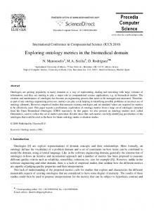
for searching any specific word is a tedious and costly job. For this reason research has been emphasized on word-spotting. This technique can be defined as the :”localization of words of interest in the dataset without actually interpreting the content” [1], and the result of such a search could look like the result shown in

Fig. 1 (without transcription). These figures (Fig. 1) demonstrates a layman’s view of the word-spotting outcome of the system.

(b) Query word for Parzival dataset

D

(a) Query word for GW dataset

(d) Sample page of GW dataset

(e) Sample page of Parzival dataset

(c) Query word for CESR dataset

(f) Sample page of CESR dataset

Figure 1: Example of word-spotting outputs (marked by rectangular boxes in (d), (e), (f)) corresponding to queries ((a), (b), (c)) from document images extracted from 3 different datasets (see Section 4)1 . The spotted query words on the complete document page are marked by a rectangular box.

A popular way to categorize word-spotting techniques is to consider those that are based on query-by-

example and those that are based on query-by-string. In the former category, a region of a document is 1

For a detailed description of the datasets, please see the experimental evaluation section 4 For a detailed description of the Parzival dataset, please see: http://www.iam.unibe.ch/fki/databases/iam-historicaldocument-database/parzival-database

2


3

defined by the user, and the system should return all of the regions that contain the same text region, that is the same as the region defined by the user. These are often achieved by learning-free, image-matchingbased approaches. For approaches that belong to the query-by-string category, queries of arbitrary character combinations can be searched. These approaches require a model for every character. Consequently, they are often achieved by learning-based approaches, such as HMM [2, 3] or a Bidirectional Long Short-Term Memory (BLSTM) neural network [4] . These approaches allow us to obtain very good performance when the learning set is representative of the writing/font styles that are found in the document to be searched. The

ra ft

well-known drawback of learning-based approaches is the requirement of a set (most often enormous) of transcribed text line images for training, which could be costly to obtain for some of the historical datasets.

Only very few approaches appear to be able to work with a low level of training data [5, 6]. Moreover, the training (transcription of the learning set and learning of models) could have to be re-performed for new documents depending on the variability of the writing/font styles. Thus, if neither the language nor

the alphabet of a historical document are known or if creating a new learning set and retraining the system is necessary but not possible, a learning-free approach to word-spotting might be the only option that is available. Consequently, a fair comparison between the two approaches is difficult to perform without

including these criteria and we decided in this study to focus on learning-free approaches. These approaches can be further categorized depending on the level of segmentation that is used.

Segmentation-Based Word-Spotting methods: The concept of word-spotting as the task of detecting

words in document images without actually understanding or transcribing the content, was initially the subject of experimentation by Manmatha et .al. [1]. This approach relies on the segmentation of full

D

document images into word images. A general and highly applicable approach for comparing word images

is to represent them by a sequence of features, which are extracted by using a sliding window. These word images can be thought of as a 2D signal, which can be matched using dynamic programming [1, 7] based approaches. Some methods that were oriented toward bitwise comparison of images were also investigated [8], as well as holistic approaches that describe a full image of words [9, 10]. An approach based on lowdimensional, fixed-length representations of word images, which is fast to compute and fast to compare, is proposed in [11]. Based on the topological and morphological information of handwriting, a skeleton based graph matching technique is used in [12], for performing word-spotting in handwritten historical 3


4

documents. There have also been some attempts to spot words on segmented lines to avoid the problems of word segmentation. Indeed, depending on the document quality, line segmentation could be comparatively easier than word segmentation. The partial sequence matching property of CDP [13] is one possibility. Using over segmentation is also an alternative as in [14], where the comparison of sequences of primitives obtained by segmentation and clustering (corresponding to similar characters or pieces of characters) is investigated. The necessity of proper word segmentation (or line segmentation in some cases) and the high computa-

ra ft

tional complexity of matching are critical bottlenecks of most of the techniques in this category. Moreover, these techniques are prone to the usual degradation noise that is found in historical document images. Most of them cannot spot out-of-vocabulary words.

Segmentation Free word-spotting methods: In [15], the authors proposed another type of matching

technique, by comparing based differential features to match only the informative parts of the words, which

are detected by patches. A common approach for segmentation-free word-spotting is to consider the task as an image retrieval task for an input shape, which represents the query image [16]. For example, a HOG

descriptors based sliding window is used in [17] to locate the document regions that are the most similar

to the query. In [18], by treating the query as a compact shape, a pixel-based dissimilarity is calculated between the query image and the full document page (using the Squared Sum Distance) for locating words. A heat kernel signature (HKS) based technique is proposed in [19]. By detecting SIFT based key points on

the document pages and the query image, HKS descriptors are extracted from a local patch that is centered at the key points. Then, a method is proposed to locate the local zones that contain a sufficient number of

D

matching key points that corresponds to the query image. Bag of visual words (BoVW) based approaches

were also used to identify the zones of the image that share common characteristics with the query word. In [20], the Longest Weighted Profile based zone filtering technique is used from BoVW to identify the location of the query words in the document image. In [21], local patches powered by SIFT descriptors are described by a BoVW. By projecting the patch descriptors to a topic space with a latent semantic analysis technique and compressing the descriptors with a product quantization method, the approach can efficiently index the document information both in terms of memory and time. Overall, segmentation-free approaches can overcome the curse of the segmentation problems, but they have comparatively low accuracy (in comparison 4


5

with segmentation-based and learning-based approaches) and a high computational burden, considering the full image regions as an apparent candidate for matching. Table 1: Grouping of state of the art techniques of word-spotting

Segmentation Free Line Based Word Based Character Based

Without Learning [15, 16, 17, 18, 19, 20, 21] [13], [Proposed Method] [1, 7, 8, 9, 10, 12], [Proposed Method] [14]

With Learning [2, 3, 4, 5, 6]

ra ft

The Table 1 summarizes several existing word-spotting methods depending on the criteria mentioned above: learning or not; and level of segmentation. From this literature review, we noticed that there are still some important unresolved problems in this domain, e.g., word-spotting independent of script and language

variability, has not been properly addressed by the research community. Additionally, excluding learning based approaches, there are few research studies that could handle noise and degradation effects in histori-

cal documents [22, 3]. In most languages, there are several variations or derivatives of words that could be interesting for the user. For example, the French word cheval (horse) can have derivatives such as ”cheva-

lerie”, ”chevaux”, ”chevalier”. In old French, lexical variations also exist e.g., ”cheual”,”chevaus”, and these variations do not change the meaning of the word; being able to retrieve these derivatives of the word that is being searched could be very useful. However, very little work is available in this direction as well as in the direction of skipping prefix and suffix of segmented words [13, 7].

For this reason, in this paper, we propose a robust learning-free word-spotting method by introducing a

novel sequence matching technique, called Flexible Sequence Matching (FSM). The proposed FSM tech-

D

nique is designed to overcome the bottlenecks of the other sequence matching techniques that have been applied in the domain of word-spotting, e.g., DTW [1], CDP [13], and some modified version of classical

DTW [7]. The proposed algorithm is capable of handling (to some extent) the local degradations and noise that is present in the image by skipping it, if necessary. To an extent, it can also handle lexical variations or derivatives by skipping unnecessary portions such as prefixes or suffixes. FSM is flexible with regard

to the word segmentation problem and does not truly depend on good segmentation: it can work on pieces of lines and/or on improperly segmented words (see Table 1). Finally, the approach can handle spelling

(local) variations and word derivatives. These properties allow the algorithm to find meaningful correspondences between elements of query and targets, which is not often the case for classical sequence matching 5


6

techniques. Finally, the architecture of FSM is designed in such a generalized manner that it can be easily modified into the architecture of other sequence matching techniques, e.g., Minimal Variance Matching (MVM) [23], DTW [1], Subsequence DTW (SSDTW) [24], and Continuous Dynamic Programming (CDP) [13]. To show the usefulness of FSM in the word-spotting domain, a comparison of FSM with other similar sequence matching techniques such as DTW, SSDTW, MVM, Objective Bijection Matching (OSB) [25], and CDP is performed. The remainder of this paper is organized as follows. In Section 2, a comparative discussion of state-

ra ft

of-the-art sequence matching techniques is given. The proposed word-spotting framework, along with descriptions of the used features is briefly mentioned in Section 4.1. The core idea of the paper, the Flexible Sequence Matching technique, is explained in Section 3, including it’s theoretical description, pseudo-code

and generalization properties (see Appendix E). The experimental evaluation is described in Section 4, and conclusions and future work are described in Section 5.

2. Bird’s Eye View of Sequence Matching Techniques

Many studies have been published in the literature [1, 7], following an architecture for word image

matching that is similar to the architecture that is based on classical DTW [24] (see also section 4.1). The main idea of DTW is to calculate the distance between two time series by summing up the distances of their corresponding elements. DTW yields an optimal (order preserving) relationship R of all of the elements of sequence x = {x1 , x2 , x3 ....x p } to all of the elements of sequence y = {y1 , y2 , y3 ....yq }. Dynamic programming

D

is used to find the best corresponding elements (see Annexe B for more details). It has been shown in the literature that the DTW distance is superior to the Euclidean distance [26]. This proposition has also been

proven for word-spotting [27]. Nevertheless, there are some limitations to classical DTW, especially that each element of x1..p must correspond to some y1...q , and vice versa (one-to-one, one-to-many and many-to-

one matchings). This hard constraint often forces DTW to perform a correspondence with noisy elements, which could disturb the matching and also increase the final distance value. Hence, the final ranking of the elements for the task of word-spotting can be disturbed. A critical problem arises, when sequence x 0

0

corresponds to only a part y of the sequence y: DTW can-not ignore the elements that do not belong to y . To perform partial matching of the sequences, some research has been introduced in the literature, e.g., SSDTW 6


7

[24], which is designed to find a continuous subsequence within a longer sequence that can optimally fit the shorter query sequence. Another DTW-based modification, called as DTW with corresponding window (DTW-CW) [23], can perform partial sequence matching, while using a sliding correspondence window of the same size as the query sequence and using DTW at each position. Although this approach can give better accuracy for subsequence matching, it is also very time consuming, due to it’s architectural constraint. Moreover, deciding the threshold for sliding the corresponding window is highly data dependent and a cumbersome process. Continuous Dynamic Programming (CDP) [13] is another alternative to operate

ra ft

partial matching that is showing promising results. It is similar to DTW-CW but does not need to recompute DTW at each position. It is using a specific DP-path and the minimum of output function along target

signal is giving candidate positions (see Appendix D). These partial matching algorithms have similar

drawbacks to DTW, especially considering difficulty to find relevant correspondences because of inability to skip outliers inside matched part. Moreover correspondences between elements is not directly provided with output.

To handle noisy points in DTW, derivative DTW (DDTW) was proposed in [28]. This method is based

on derivatives of feature elements, instead of the original feature sequence. An useful modification of the classical DTW technique is weighted DTW (WDTW) [29]. This approach penalizes points that have a higher phase difference between a reference point and a testing point, to prevent minimum distance dis-

tortions that are caused by outliers. In Weighted Derivative Dynamic Time Warping (WDDTW) [29], the penalization idea in WDTW is extended to DDTW to capture the benefits of both approaches. These above defined techniques, try to limit the effects of noisy elements in the sequence, but they are unable to com-

D

pletely skip the noisy elements. To address this restriction, some other sequence-matching algorithms were proposed.

To find an optimal correspondence between two sequences, a popular approach is the Longest Common

Subsequence (LCSS) [30]. Given a query and a target sequence, LCSS determines their longest common subsequence, i.e., the sequence that best corresponds between the original sequences. The dissimilarity measure is based on the ratio between the length of the longest common subsequence and the length of the whole sequence. The elements of the subsequence do not need to be consecutive points, which could be a problem for word-spotting. The order of the points is not rearranged, and some points can remain 7


8

unmatched. To make LCSS efficient, one must also set the threshold that determines when the distances between corresponding points would be treated as being equal. Determining this threshold value is a difficult task and it is highly data dependent [31]. To overcome this problem, Minimal Variance Matching (MVM) was proposed by Lateki et. al. [23]. MVM combines the strength of both DTW and LCSS, while overcoming their constraints. MVM calculates the sequence similarity directly based on the distances of corresponding elements. MVM also tries to find an optimal path including all the corresponding pairs but MVM is able to skip outliers in target during

ra ft

the matching process (see Appendix C). The notable difference between LCSS and MVM is that LCSS

optimizes the length of the longest common subsequence, while MVM optimizes the sum of distances of corresponding elements (without any distance threshold). Moreover, LCSS can skip both query and target elements, whereas MVM can skip only the target sequence. Thus, MVM could be used only when the query sequence is smaller than the target sequence, and it is useful to find the query in a larger target sequence. For

the case of word-spotting, this case is the classical situation, if we consider that the query image is rightly selected and there is no disturbing noise present in the query image. However, when there are outliers

in the query sequence and skipping those outliers from the query sequence is necessary, then the MVM properties remain limited. Finally, both algorithms (LCSS and MVM) are capable of performing one-

to-one correspondences (many-to-one and one-to-many matchings are not allowed). Another algorithm, designed by Lateki et. al. [25], is Optimal Subsequence Bijection (OSB) [25]. The goal of OSB is to 0

0

0

0

find subsequence x from x and y from y such that x best matches y , by skipping some elements from

x and y because both the sequences might contain some outlier elements. Thus, the properties of OSB is

D

more similar to the properties of LCSS. To prevent skipping too many elements, the algorithm introduces a penalty for skipping 2 . Like MVM, OSB can perform only one-to-one correspondences, both of these algorithms cannot do many-to-one and one-to-many correspondences. But the noteworthy point is that OSB has a much higher computational complexity than MVM.

The Tables 5 and 6 in Annexe A, summarize the main properties of these different algorithms. We can

see that none of them include at the same time the main properties that are necessary for word-spotting, i.e., being able to perform multiple matches because signals (query and target images) could have local 2

Please note that, the MVM algorithm does not have any penalty for skipping

8


9

stretching/extension and because of varying writing/font styles; being able to operate partial matching by skipping irrelevant elements at the beginning and end of the target because of wrong segmentation; and being able to skip noisy elements inside the target because of lexical variations or degradations. For this reason, we propose, in the following section, a novel sequence matching algorithm. This algorithm can successfully overcome most of the problems of the aforementioned individual sequence-matching algorithms and thus could be very useful for the word-spotting domain as well as many other applications for which

ra ft

such flexibility is required.

3. Flexible Sequence Matching (FSM)

In this section, the complete mathematical structure of FSM is described. The main properties of FSM

are summarized in Tables 5 and 6. FSM creates a relation R from two finite sequences x (query) to y (target),

of different lengths p and q: x = (x1 , x2 , ....., x p ) and y = (y1 , y2 , ....., yq ); p ≤ q.3 The goal of the algorithm 0

0

0

is to find y (y ⊂ y) such that x best matches y . The relationship R, is performed on the set of indices

{1, ....p} × {1, ....q}, where, one-to-one, one-to-many and many-to-one mapping is possible. Then, based on the correspondence, a distance between the two sequences is computed. 3.1. Theoretical Description of FSM

The theoretical background of the FSM algorithm comes from DTW and MVM techniques. From

DTW, we are mainly keeping its relational structure (one-to-one, many-to-one and one-to-many matching

in order preserving manner). From MVM, we kept its algorithmic structure so that the participation of all

D

the elements of y in the relation R could be relaxed. It means, if there are some noisy elements present in y then, they can be intelligently skipped by the algorithm. In the following, a stepwise description of

FSM algorithm is illustrated. Note that, 1D time series signals are considered for ease of description but the extension to sequences of elements corresponding to vectors of same dimension, can be easily performed. q First, the difference matrix D is calculated by using the Euclidean distance Di, j = (y j − xi )2 ; 1 ≤ i ≤ p; 1 ≤ j ≤ q. According to [23], there is no restriction on using various distance measures and any of the 3

The length of the query sequence should always be less than or equal to the length of the target. For an application, if this constraint is not the case, then we can consider only the query to the target and vice versa, i.e. we simply reverse the order of the input arguments in the FSM function.

9


10

distance measures can be considered. Here, D can be used to generate a directed acyclic graph (DAG), denoted as G, where each of the elements of D can be considered to be a node. The links between each node and it’s child nodes are obtained by solving a shortest path problem, i.e., by using the cost function H defined in (1), where Du,k represents the parent nodes, and Di, j represents the child nodes.4 ( Di, j if i = u + 1 and k ≤ j ≤ L (i); if i = u and j = k + 1 (ii) H(Du,k , Di, j ) = ∞ otherwise L = (k + 1) + elasticity − |k − u|; elasticity = |q − p|

(1) (2)

ra ft

In (1), any node Du,k has the flexibility to be connected with another node Di, j in two possible ways. Here, (i) means that, a parent node can be connected with child nodes in the next row (i = u + 1), in the same

column or at the right (k ≤ j ≤ L), up to a given user-defined elastic limit L, with respect to the position of

parent node.5 This elastic limit represents the number of jumps that could be performed inside the matched

part of the target. By default, it is equal to the difference in size, between the query and target sequences (i.e.

|q − p|) minus the number of jumps already used (i.e., the difference between the column and row indexes of

the parent node: |k − u|)6 . The connection at the same column (k = 1) is mainly to ensure the many-to-one

matching (link with the parent node and the child node in the same column). The condition (ii) says that

the parent node can also be connected with the node next to it, in the same row. This particular connection, ensures the one-to-many matching facility. In this way, we can generate G (see Fig. 2). / Pattern Recognition 00 (2015) 1–42

D1,2

D2,1

D2,2

D3,1

D3,2

...

D2,L

...

Dp

1,1

D p,1

D1,q

...

D2,L+1

D2,q

...

D

D1,1

20

D3,q

...

Dp

D p,2

1,2

...

...

...

Dp

...

1,q 1

D p,q

1

Dp

1,q

D p,q

Figure 3: DAG constructed using a distance matrix obtained from two sequence. Figure 2: DAG constructed using a distance matrix obtained from two sequence.

It is noteworthy to mention that, in certain application, many-to-one and one-to-many characteristic of

FSM may not be required. In such cases, the last two terms of Eq3b, could be ignored. The path cost P(i, j)

Judging the intensity of the noise, that is present in the signal is a difficult and puzzling problem. Inis updated only when there is a shorter path coming from a parent node. The optimal structure condition guarantees that the returned matrix P, contains the cost of the shortest path leading to every node.

4

The distance comparable sequences can be by getting the minimum value stored Please note that the indexes of allbetween of thetwo matrix notations used in obtained this paper, always start from 1. When q = p, the value oflast elasticity takenof to becost 2 to maintain facility. at the row and lthis column path matrix P, wheresome p  l skipping q. To normalize the sequence dissimi6 This constraint is notlarity mandatory but ititlimits the complexity of pairs the algorithm. value8 , we divide by the number of corresponding between the target and query sequence

5

10

5.2. Description of the Proposed Pseudo Code As an output, the algorithm provides the path costs in P along with two other matrices (R and C ), which are used to backtrack the shortest path, giving the closest correspondence between query and target elements. The matrix R keeps track of rows and C keeps track of column and the array W merge these indexes to get the path. The overall process is given by Algorithm 1. The first row of P is obtained by Eq3a. All the other cells of P are initialized with infinity. The cells of the path cost matrix (P) are calculated (refer to lines 4 27) by iterating i over each row where k iterates over parent nodes at row before (i-1) and j keeps


11

deed, deciding, whether a specific element should be considered to be an outliers (hence skipping it) or not is not straightforward. For example, in the case of LCSS, the user must define a threshold. In FSM, this type of threshold is not required, but the system cannot be allowed to skip outliers without any resistance. Otherwise, the process can frequently skip elements, instead of matching them with some acceptable dissimilarity cost. Thus, to limit skips, skipCost is introduced. This cost corresponds to a distance value that is higher than the cost that corresponds to an acceptable distance between corresponding elements. Due to the dependency of the skipCost value on the dataset, we estimate this value in the following way. We randomly

ra ft

choose two query sequences. For each, we randomly choose two corresponding targets that should match.7

Then, the distance matrices between the chosen queries and targets are calculated. A vector Mi is created to

contain the average of the top m minimum values from each row i, i = 1, ..., p of the corresponding matrices. The obtained vectors Mi for each query and target pair are merged together and sorted in ascending order, 0

giving Mmerged . Then, only 90% of the elements of Mmerged are kept in Mmerged . These values correspond

to the distances between the matching elements.8 Finally, skipCost is computed based on the mean and 0

standard deviation of Mmerged (see (3)). ∀ii=1,...,p ,

0

0

Mi = mean{top-m min(Di, j )}; S = skipCost = mean(Mb merged ) + 2 × std(Mb merged ) (3) j=1,...,q

To perform the matching, we must find the shortest path through G from a single initial node D1, j ,

which leads to D p,l ; l ∈ {p, ..., q}. It is obtained due to a path cost matrix P(i, j); 1 ≤ i ≤ p; 1 ≤ j ≤ q and

satisfies the following conditions:

i) starts at the 1 st row between column 1 and q; this starting point allows us to skip an unnecessary prefix.9

D

ii) ends at the last row p in a column l ∈ {p, ..., q} to skip an unnecessary suffix.

iii) the shortest path between each pair of reachable nodes in G can be found from P.

The construction of P(i, j) is given by (4a-c). (4a) says that the 1 st row of the distance matrix D is copied to the path cost matrix P. Each cell that belongs to the ith row (i ≥ 2) is calculated by first choosing the 7

Choosing such elements can be viewed as a calibration step that is not time consuming or difficult. The idea of choosing m minimum values is to have a cost that will not be null, when perfect matches are available between the query and target sequences. Here, m = 2 is the minimum to consider, but experimentally, taking m = 5 is less sensible and is in an acceptable range, with respect to the sizes of our sequences. It should be noted that this parameter value is not very important for the proposed algorithm. 9 Please note that to allow substring matching, these skips at the beginning and end are not penalized, i.e., no skipCost is added 8

11


12

possible parent nodes in a previous row (i − 1) and in the columns k that range from ((i − 1) − elasticity) to ((i − 1) + elasticity) (see (4c)). Considering a parent node, its child nodes can belong only to the next row and in columns that range from the next column (k + 1) until column (k + 1) + elasticity − |k − (i − 1)|. Other possible links are for many-to-one and one-to-many matchings: the vertical link (from node (i − 1, j) to (i, j)) is responsible for many-to-one matching and the left link (from (i, j − 1) to (i, j)) is responsible for merged0

one-to-many matching. Please note that in such cases, a small penalty (C = mean(Mi

)) is introduced

to limit the numbers of multiple matchings. If, for some application, multiple matching is not required,

ra ft

the last two terms of (4b) can be ignored.10 The path cost P(i, j) is updated only when there is a shorter path that comes from a parent node. The optimal structure condition guarantees that the returned matrix P, contains the cost of the shortest path that leads to every node under the previous constraints. P(1, j) = D1, j if 1 ≤ j ≤ q o    n   P(i − 1, k) + Di, j + (S × ( j − (k + 1)))        if L P(i, j) =  min  {P(i, j − 1) + C + Di, j }       {P(i − 1, j) + C + Di, j }   {2 ≤ i ≤ p}  L =  max[1, (i − 1) − elasticity] ≤ k ≤ min[q, (i − 1) + elasticity]  k + 1 ≤ j ≤ min(q, (k + 1) + elasticity − max(0, |k − (i − 1)|))

(4a)

(4b)

   

(4c)

The distance between two comparable sequences can be obtained by obtaining the minimum value that

is stored in the last row at the lth column of the path cost matrix P, where p ≤ l ≤ q. To normalize the

sequence dissimilarity value, we divide it by the number of corresponding pairs between the target and query sequence.

D

3.2. Description of the Pseudo Code

As an output, the algorithm provides the path costs matrix P along with two other matrices, (R and C ),

which are used to backtrack the shortest path, giving the closest correspondences between the query and target elements. The matrix R keeps track of the rows and C keeps track of the columns, and the vector W merges these indexes to obtain the final path. The overall process is given by Algorithm 1. All of the cells of P are initialized with infinity. Next, the first row of P is obtained by (4a) (lines 2 − 3). The other cells are calculated (refer to lines 4 − 25) by iterating i over each row, while k iterates over the parent nodes in

10 One should note also that the elements of the path can be weighted as in DTW’s variants. This was done in our implementation (see section below) but is not mentionned here for clarity.

12


13

Algorithm 1: Flexible Sequence Matching Input: x1...p , y1...q , D pq (double × double), elasticity(= |q − p|), S(double), C(double) ¯ Output: P pq (double × double), W(vector < (int, int) >), d(double) 1 P←∞ . Initialize all the cells of P matrix by ∞ 2 for j ← 1 to q do 3 P(1, j) ← D(1, j) . Fill the 1 st row of P with the 1 st row values at D matrix 4 5 6 7 8

ra ft

9

for i ← 2 to p do if i = 2 then R←q . Complete flexibility is given for choosing the 1 st node L←1 else R ← min(q, (i − 1) + elasticity) L ← max(1, (i − 1) − elasticity)

10 11 12 13 14 15 16 17

for k ← L to R do D ← ((k + 1) + elasticity) − max(0, {k − (i − 1)}) for j ← k to D do if j = k then J ← C; W ← 1 . Penalty and weights for vertical links else if j = k + 1 then J ← 0; W ← 1 . No penalty/weights for diagonal links else J ← 2/3 × { j − (k + 1)} × S; W ← 1/3 × { j − (k + 1)}; . Penalty proportional to number of jumps if P(i, j) > (P(i − 1, k) + W × D(i, j) + J ) then P(i, j) ← (P(i − 1, k) + W × D(i, j) + J ) . Link between two rows R(i, j) ← i − 1; C (i, j) ← k if P(i, j) > P(i, j − 1) + C + D(i, j) then P(i, j) ← P(i, j − 1) + C + D(i, j) . Link from left node R(i, j) ← i; C (i, j) ← j − 1

18 19

20 21 22 23 24

25

I = argmin P(p, t) p≤t≤q

. Column index (from index p to q), of last row with the minimum value

D

26

27

28

29

30

31

32

r = p; c = I; cnt = 1 while ((r ≥ 1)&(c ≥ 1)) do Wcnt = (r, c) . Storing the cell indexes in the array for getting the warping path t = C (r, c); r = R(r, c); c = t; cnt + + reverse(W) . The warping path vector is reversed to get elements in right order P p,I P p,I ¯ i) d = |W| ; where |W| = sizeo f (W) ii) d¯ = |W|+{{W(cnt−1,1)−1}+{q−W(1,1)}} . Depending on the ¯ requirement, the normalized final distance (d) can obtained in two different ways.

the row above (i − 1), and j keeps track of the child nodes for a given parent node. For each cell of each

row, first the range of the parent nodes is calculated (lines 5 − 10). When i = 2, the parent nodes can be 13


14

at anywhere in the first line/row, to allow the skipping of the irrelevant part (at no cost) at the beginning of the target. Next, for each parent node from L (left) to R (right), the possible connections with child nodes are calculated by j, which is iterated between k and D according to (4c). Similar to DTW, FSM can perform multiple matches: many consecutive elements of the query to one element of the target (line 14) and one-to-many (lines 23 − 25). It can also skip some target elements. Recall here that the jump cost (J ) is based on the number of skips that are already taken (term ( j − (k + 1)) in line 19) and the skip cost (S). Notice also that this jumping facility is here weighted in the similar way as it is in CDP (2/3 of the cost

ra ft

for reaching parent node and 1/3 for matched element D(i, j)), since preliminary experiments have shown

better results in such case. In contrast, when the parent node at (i − 1, k) is connected with the node at (i, k + 1) (diagonal link), which means that two consecutive elements of the query are matched with two consecutive elements of the target sequence, then no cost is added. The calculation of the warping path W is

given in lines 26 − 30. Initially, the index of the column, which ranges from p to q, and contains a minimum

value in the last row of the path cost matrix is found. Then, back-tracking is performed through the while loop to obtain W = W1 , W2 , W3 , ..., Wk , ...WK ; max(q, p) ≤ K ≤ q + p − 1, where Wk contains an ordered set

of indices of the corresponding elements. Finally, the distance d¯ (see line 32 of algorithm 1) is outputted. 3.3. Properties of FSM

The warping path of FSM follows these constraints:

i. Boundary Condition : FSM does not maintain the boundary condition of classical DTW and can

perform partial sequence matching. The warping path can start from any specific column in the last

D

row, ranging from the index p to q, i.e., WK = (p, t); p ≤ t ≤ q and the warping path can end at any column, in the first row, i.e., W1 = (1, u); 1 ≤ u ≤ q.

ii. Continuity Condition : The continuity condition of classical DTW is also not exactly maintained by FSM: Wk = (a, b) is followed by Wk+1 = (a0 , b0 ); where (a0 −a) ∈ [0, 1] and (b0 −b) ∈ [0, 1, ...|p−q|+1].

Due to this characteristic, FSM can jump outliers from the target signal.

iii. Monotonicity Condition : The monotonicity condition restricts the warping path from going back in time: Wk = (a, b), Wk+1 = (a0 , b0 ) is constrained by (a0 − a) ≥ 0 and (b0 − b) ≥ 0.

Additionally, it is very easy for the presented algorithm to be changed in such a way that it can behave as other algorithms such as DTW, MVM and SSDTW (details can be found in Appendix E). 14


15

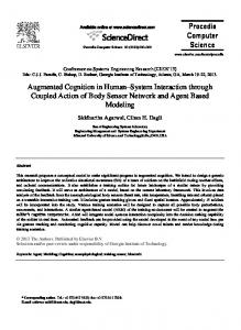
3.4. Examples of matching with FSM Using some toy examples, the behavior of FSM, compared to DTW and MVM is demonstrated in Fig. 3. Figs. 3a, 3b and 3c are showing the results of matching the sequences: Q = [1, 2, 8, 8, 8] and T = [1, 2, 9, 95, 79, 26, 39, 31]. It can be seen that for the case of DTW, the 1 st , 2nd and 3rd elements of the query and target are correctly matched. However, the 4th element (0 80 ) of the query is forced to be matched with the 4th element (0 950 ) of the target. The last element of the query is also forced to be matched with the other remaining elements of the target (many-to-one matching), which significantly increases the final

ra ft

distance. The MVM algorithm can improve the matching process by skipping the outliers elements 0 950 and 0 790 .

However, it’s inability to have many-to-one matching and it’s restriction on the numbers of matched

elements (which should be equal to the number of elements in the query), compel the algorithm to match the 4th and 5th elements of Q with the 6th and 8th elements of T . In contrast, it can be easily visible that

FSM can overcome these restrictions and provide correct correspondences. In such a case, small costs will minutely penalize the final distance for the one-to-many matchings.

In Figs. 3d, 3e, and 3f, the same trends can be seen. However, here we can see that even if the lengths

of the target and query signals are same, the elasticity for the FSM algorithm is taken to be 2, which allows

it to skip outliers inside the target. DTW cannot do that, and neither can MVM, in such a case. Figs. 3g, 3h, and 3i illustrate the same possibilities when the query is smaller than the target. In such a case, MVM

D

behaves the same as FSM. Again, DTW is forced to match all of the elements.

(a) Partial matching ability of DTW

(b) Partial matching ability of MVM

(c) Partial matching ability of FSM

(d) Multiple matching ability of DTW (e) Multiple matching ability of MVM (f) Multiple matching ability of FSM

(g) Skipping ability of DTW

(h) Skipping ability of MVM

(i) Skipping ability of FSM

Figure 3: Partial matching, many-to-one and one-to-many matching and noise skipping ability of DTW, MVM and FSM.

15


16

3.5. Time complexity of FSM The worst case complexity of FSM is calculated by computing total number of possible parent nodes at each row of P matrix. In worst case, we would have a subset of at most {(2 × |q − p|) + 1} parent nodes (see line 9, 10 of Algorithm 1) at each row of P(i, j)(1 ≤ i ≤ p; 1 ≤ j ≤ q) matrix; which indeed can be represented as the vertices of DAG G. Then for each of the parent nodes in row i is linked to at most T child nodes. Since there are total p rows, the algorithm complexity could be defined by: [p×{(2×|q− p|)+1}×T ]. (5)

ra ft

T = [{( j + 1) + |q − p|} − ( j + 1)] + 1 − ( j − i) + 1 + 1 = |q − p| + ( j − i) + 3 ≈ |q − p| + 3

In Eqn 5, the term ( j − i) can be ignored (it reduces the complexity) for performing worst case analysis.

The term 3 comes from adding the diagonal link, link with the right child node on the same line as parent

node and the child node just below parent node (see line 14 of Algorithm 1). The worst case complexity of FSM is Θ([|q − p| + 3] × [p × {(2 × |q − p|) + 1}]) = Θ(2.p × ((|q − p| + 2)2 − 1)) ≈ Θ(2.p × (|q − p| + 2)2 ).

This assumption is also true : Θ((2.|q − p|2 ).p) < (Θ(2.q2 .p). Furthermore the complexity can be reduced

to linear (Θ((2.|q − p|2 ).p) ≈ Θ(p) when q ≈ p; i.e. matching whole target)). The time complexity of

FSM can further be reduced by introducing an admissible lower bound. However, in this work we focus on demonstrating the utility of FSM; we will address speedup and index-ability of FSM in future work.

4. Experimental Evaluation

The experiments of the word-spotting application was performed on: i) correctly segmented words,

D

ii) incorrectly segmented words, i.e. pseudo-words, iii) correctly segmented lines. Indeed, depending on the characteristics of the documents, it can be comparatively easier to perform word segmentation or line segmentation. For example, if inter-word gaps are not large enough or are variable (which is often the case in old historical documents), word segmentation can be very difficult. However, for handwritten documents with curved and touching lines, segmenting pieces of lines could be easier. The level of difficulty is highly

writer and language dependent.11 Thus, due to the pros and cons of the two segmentation techniques, we have performed experimental evaluations on all cases. 11

Please note also that an advantage of line segmentation is that it can be possible to spot hyphenated words that span onto two

lines.

16


17

Offline Feature Extraction Each image

All document images

Binarization and De-noising

Segmentation of word based on RLSA (optional) Feature extraction and offline feature storage into data file (.dat)

FSM Matching

Noisy border removal

Text line segmentation based on projection profile

RLSA threshold estimation Connected Components labeling

Feature extraction

ra ft

Query image

Lines/words ranked according to score

Figure 4: (a) The block diagram of the proposed word-spotting system.

4.1. Word-spotting Framework

In this section, our complete word-spotting framework is briefly explained in a stepwise manner. Be-

cause the main scope of this paper is a word image ”matching technique”, we have not provided the details about all of the steps of the word-spotting process but only the main ones. This word-spotting architecture is very common and has been used by several researchers [1, 7]. It is illustrated in Fig. 4. 4.1.1. Image preprocessing and pseudo-word segmentation

First, we must pre-process each of the scanned document pages. To binarize the documents, we used

the adaptive binarization technique proposed in [32]. Due to improper scanning, document images might be

D

framed with unwanted text areas of the neighboring pages. Thus, after binarization, we apply the technique, described in [33], for obtaining proper text boundaries. Then, the text regions are segmented into either lines or pieces of lines, up to words or parts of words. Indeed, due to the properties of FSM, we do not require precise word segmentation. The textual elements obtained are called here ”pseudo-words”. Word segmentation could be obtained by using Run Length Smoothing Algorithm (RLSA) based tech-

niques. This can provide good results for high quality printed documents, but the results could be poor when inter-word spaces are variable which is often the case in handwritten documents as well as in historical printed documents. Thus, applying Horizontal RLSA (H-RLSA) with adaptive threshold [34] is a better solution. This threshold actually defines the average inter-character gap in a word, and it inherently depends 17


18

on the considered dataset. To obtain it automatically, a preliminary text line segmentation is performed on the document pages. Proper segmentation of all of the text lines is not required in this case. We need to have only some prominent segmented text lines, which can help us to understand the inter-character gaps as well as the inter-word gaps in a text line. Thus, the basic text line segmentation algorithm based on the projection profile [34] is used here, and only the best segmented lines (based on the heights of the segmented text lines) are considered. Then, the average inter-word character gap is obtained from the histogram of gaps between connected components. Afterward, that H-RLSA is performed on the image by using the average character

ra ft

gaps as a threshold for obtaining the pseudo-words (words that are not necessarily well segmented). 4.1.2. Feature extraction

After obtaining pseudo-words (or lines), the next task is to extract features from them. Features are

extracted from gray scale and also binary normalized images. In the following, we describe two different

categories of features, namely column based features and a histogram of gradient-based features. Once the features are extracted, they are stored off-line for faster retrieval.

Table 2: Extracted features from the word images, considering an image with N columns and M rows

Feature description Sum of foreground pixel intensities in pixel columns (from greyscale image) Number of background-to-ink transitions in pixel columns Upper profile of sequence (top most position of ink pixels in pixel columns) Lower profile (bottom most position of ink pixels in pixel columns) Distance between upper and lower profile (in number of pixels) Number of foreground pixels in pixel columns Center of gravity (C.G.) of the column obtained from the foreground pixels 1 ≤ n ≤ N  P M 1  [ ρ m=1 m i f wb (m, n) = 1]; ρ , 0; ρ = No. o f f oreground pixels at nth column;  F7(n) =   t Obtained by interpolation; ρ = 0

D

Feat. Nb. F1 F2 F3 F4 F5 F6 F7

F8

   1     F8(n) =      t

Transition at C.G. obtained from F7 wb (F7(n), n) = 0; and wb (F7(n − 1), n) = 1 or wb (F7(n), n) = 1; wb (F7(n − 1), n) = 0 Obtained by interpolation

Column-based features : A set of statistical column based features, which have been used previously

for handwriting recognition is broadly described in [35]. A subset of these features has been used by several researchers for word-spotting [1, 4]. One should notice that, these features are mostly based on the binary image, so they are not much sensitive to illumination variations, provided that the used binarization 18


19

technique has taken into account the issues related to illumination variations, which is the case here with [32]. But some of these features are sensitive to the local noise, especially F1 , F2 , F6 . Although the column based features can be improved, selected, or outperformed in terms of accuracy by more complex features ( e.g. gradient-based features [36], or graph similarity features [37]), due to their lower computational cost, they remain quite interesting and we chose not to focus on this point in this study. Here, we have chosen 8 features, F1 , F2 , . . . , F8 to describe each sequence using pixel column information. For an image with a width of N pixels, a sequence of N vectors in 8 dimensions is obtained by moving

ra ft

from left to right. A description of the features is given in Table 2. Among them, features F1− F6 have been used several times in the literature [1], [4], [36], [38], but the features F7 and F8 are proposed in this work.

F7, corresponds to the center of gravity of the foreground pixels inside a column. In the corresponding equa-

tion in Table.2, wb denotes the binarized version of the word image, m represents the row coordinate and n

the column’s coordinate. For columns that have no foreground pixels, F7 is calculated by nearest neighbor interpolation, with the help of the neighboring columns having foreground pixels. F8, which is calculated by

using the location of the center of gravity (obtained from F7), is the number of transitions, from foreground to background (1 to 0) or from background to foreground (0 to 1) at these calculated centroid locations of pixels.

Slit style HOG based features : Slit style HOG (SSHOG) features were pri-

marily introduced in [13]. We used the same features for some experiments

in order to compare various approaches. HOG based features are less sensi-

D

tive than column based features considering noise and illumination variations because they do not need binarization and they are based on gradients of the image. For calculating this feature, a fixed sized window is slided over the image in a horizontal direction to extract the HOG features from each slit. For calculating the HOG descriptors, we need to divide the slit into smaller rectangular regions (called cells) along horizontal and vertical directions. A block is defined as a group of h × w cells. Blocks are slided over each slit

Figure 5: Block normalization technique for SSHOG

that has the same width as the width of the block. The horizontal overlapping of the original HOG could be well realized by the sliding window and sequential representation of vectors. The relationships between 19


20

slits, blocks and cells are shown Fig. 5. This figure shows, three blocks (b11 , b12 , b13 ), each one composed of four cells (2 × 2), denoted by h11 ...h24. Notice here that since SSHOG features are obtained from a slit of several pixels in width, skipping one element with FSM is corresponding in fact to skipping one slit and thus several pixel columns. Such kind of side effect might need to be further studied. 4.2. Results on segmented words This expriment is performed with the George Washington historical dataset that contains 20 pages of

ra ft

letters, orders, and instructions written in 1755 by George Washington and some of his associates. Thus, obviously it inhibits some variations in writing style.The quality of the scanned pages varied from clean to difficult-to-read by humans (see Fig. 8b). This specific dataset was made by considering 10 better quality

pages among the 20. We consider 14 query images (see Fig. 8b) and the 2381 properly segmented target

words coming from the 10 pages. To perform the experiment, we used the architecture and framework

described in section 4.1 with the column-based features (see Table.2). Please note that, due to improper segmentation, some of the target words can be smaller than considered query word. In such cases, that

particular small target word is considered as query and the original query word is considered as target

word.12 The performances are evaluated using the mean average precision (mAP)13 for all of the selected

14 query words as well as Precision/Recall curves based on number of retrieved elements considered. The results, shown in Fig. 6, demonstrates that FSM significantly outperforms all other algorithms. 1.0

CDP (0.3619) DTW (0.4557) MVM (0.2026) SSDTW (0.3349) FSM (0.4991)

0.9 0.8 0.7

D

0.6

Precision

0.5 0.4 0.3 0.2 0.1 0

0

0.1

Recall 0.2

0.3

0.4

0.5

0.6

0.7

0.8

0.9

1

Figure 6: Comparative performance of CDP, DTW, MVM, SSDTW and FSM on segmented words of GW dataset.

12

In such cases, the 2nd way of normalization is used for FSM, to avoid wrongly segmented small words from appearing at top ranked positions in overall nearest neighbor ranking process. Refer to Algorithm 1, line 32. 13 https://en.wikipedia.org/wiki/Information retrieval#Mean average precision

20


21

4.3. Results on segmented pseudo-words The application of FSM on segmented pseudo-words is evaluated by an experiment on a dataset called CESR. This dataset comes from the resources of the Centre d’Etude Suprieure de la Renaissance14 , through the BVH (Bibliothèques Virtuelles Humanistes15 ) project. The CESR has a collection of precious historical books, that date from the middle of the XIV century to the beginning of the XVII century. The dataset was composed from the two volumes of Essais de messire Michel Seigneur de Montaigne, Chevalier de l’order du Roy, & Gentil-homme ordinaire de Sa Chambre. This first edition was published in Bordeaux in

ra ft

1580 by S. Millanges16 . The languages used in the books are Latin or French. All the pages were scanned

with a resolution of 312 × 312 dpi and were saved in grey-scale format (see Fig. 7). Vol.I contains 520 pages and Vol.II contains 676 pages. To build the dataset, we selected 123 relevant queries from the user’s point of view, such as those that could have lexical variations. Each query and its derivatives are grouped for evaluation: each image in a group is considered to be a query, and then, all of the other words in the group are considered to be relevant targets and must be retrieved also. For each query (and its derivatives), the research is performed with the target words, segmented from the set of full page images, in which

at least one target appears. The total number of target words in each group varies from 1700 to 21000 approximatively. The statistics are given in Table 3. 4.3.1. Experimental Setup

To perform experiments with this dataset, we used the architecture and framework, described in section

4.1. The column-based features (see Table 2) are used. Very small segmented words (e.g., one or two

D

characters) are pruned by considering their width with respect to the width of the original query word, which allows to makes experiments faster. We heuristically decided that, if the width of any target word is less than 35% of the width of the query word, then it is not considered for matching. 4.3.2. Results

Overall, the results of FSM and CDP are better than those of DTW (see Fig. 7e). The overall difference

between CDP and FSM seems not very significant (less than 0.5%) but it seems that FSM has a higher 14

http://cesr.univ-tours.fr/ See Bibliothèques Virtuelles Humanistes Project: http://www.bvh.univtours.fr/presentation en.asp 16 Please see the following links for more details about the book: https://www.lib.virginia.edu/rmds/collections/ gordon/literary/montaigne/bibliography.html and http://search.lib.virginia.edu/catalog/u50318 15

21


e◦ C¯ Q˘ ◦ N libre 19 0.712 liberte 2 0.308 librement 3 0.189 ¯ = 0.403; AF ¯ TW = 3192; AC cheualier 4 0.501 cheual 38 0.509 cheualerie 1 0.451 cheuallier 1 0.421 cheuaus 4 0.395 cheuaux 8 0.400 ¯ = 0.446; AF ¯ TW = 7570; AC

e◦ C¯ F¯ Q˘ ◦ N roy 119 0.272 0.304 royales 1 0.042 0.029 royaume 2 0.027 0.035 royaumes 4 0.038 0.037 royaus 1 0.082 0.051 royaute 2 0.116 0.068 royaux 1 0.107 0.060 royne 8 0.252 0.116 roys 17 0.173 0.145 rois 16 0.021 0.044 roistre 1 0.012 0.012 roit 20 0.017 0.038 ¯ = 0.097; AF ¯ = 0.078 TW = 20696; AC reconneut 1 0.045 0.117 reconnoi 1 0.047 0.130 reconnoissable 2 0.343 0.344 reconnoissance 6 0.318 0.358 reconnoissant 1 0.334 0.328 reconnoissent 1 0.307 0.112 reconnoissoient 1 0.219 0.258 reconnoissoit 2 0.291 0.343 reconnoissons 3 0.344 0.333 reconnoistre 7 0.140 0.174 reconnoit 5 0.052 0.184 reconnoitre 4 0.162 0.207 reconnoy 3 0.088 0.084 reconnu 2 0.044 0.172 reconnue 1 0.037 0.097 ¯ = 0.185; AF ¯ = 0.216 TW = 6117; AC

e◦ C¯ F¯ Q˘ ◦ N connoi 4 0.019 0.035 connois 5 0.312 0.329 connoissan 11 0.394 0.396 connoissance 34 0.380 0.382 connoissans 2 0.175 0.181 connoissant 4 0.401 0.324 connoisse 1 0.429 0.407 connoissent 4 0.355 0.365 connoissoit 3 0.380 0.414 connoist 1 0.276 0.371 connoistre 12 0.176 0.197 connoit 5 0.035 0.053 connoitre 3 0.043 0.047 connoy 5 0.021 0.029 connu 3 0.018 0.028 connue 1 0.031 0.029 connues 4 0.029 0.028 connus 1 0.018 0.023 ¯ = 0.194; AF ¯ = 0.202 TW = 13431; AC cognoissons 1 0.505 0.496 cognoistre 12 0.583 0.543 cognoit 6 0.147 0.112 cognoitre 2 0.371 0.441 cognosci 1 0.142 0.296 cogneu 3 0.098 0.102 cogneue 2 0.065 0.086 cogneut 1 0.121 0.095 cognoi 1 0.094 0.086 cognois 5 0.519 0.513 cognoisoit 1 0.569 0.518 cognoissan 2 0.516 0.505 cognoissance 29 0.528 0.473 cognoissances 1 0.500 0.405 cognoissant 1 0.486 0.460 cognoissent 6 0.492 0.438 cognoissions 1 0.470 0.479 cognoissoint 1 0.499 0.465 ¯ = 0.373; AF ¯ = 0.362 TW = 11024; AC despouille 4 0.721 0.656 despouiller 5 0.785 0.742 despouillera 1 0.763 0.792 depouille 1 0.754 0.746 depouiller 1 0.392 0.358 ¯ = 0.683; AF ¯ = 0.659 TW = 1647; AC

ra ft

F˘ 0.661 0.308 0.176 = 0.382 0.494 0.443 0.445 0.516 0.436 0.333 = 0.445 victoire 23 0.646 0.575 victo 1 0.593 0.510 victoi 2 0.542 0.443 victoire 23 0.646 0.575 victorieus 5 0.375 0.425 victorieux 6 0.518 0.541 ¯ = 0.553; AF ¯ = 0.512 TW = 8220; AC mortel 11 0.363 0.352 immortales 1 0.109 0.107 immortalit 8 0.301 0.283 immortel 14 0.172 0.154 immortelle 10 0.194 0.162 immortels 2 0.197 0.171 mort 28 0.071 0.087 mortale 4 0.134 0.140 mortales 1 0.107 0.120 mortalia 5 0.090 0.075 mortalibus 2 0.078 0.051 mortalite 1 0.225 0.225 morte 10 0.047 0.049 mortelle 9 0.285 0.285 mortelles 8 0.236 0.214 mortels 4 0.199 0.190 mortem 5 0.025 0.018 mortes 1 0.040 0.081 morgue 2 0.018 0.015 morti 1 0.176 0.160 mortis 3 0.032 0.028 morts 3 0.065 0.080 mortua 1 0.022 0.016 mortuum 1 0.079 0.059 mortuus 1 0.021 0.016 mortz 3 0.060 0.080 ¯ = 0.129; AF ¯ = 0.124 TW = 13518; AC

22

D

reconoissent 1 0.092 reconoissoit 1 0.104 reconoitre 1 0.055 recogneu 1 0.143 recognois 1 0.328 recognoissan 1 0.312 recognoissance 3 0.330 recognoissant 1 0.297 recognoisse 1 0.439 recognoissons 1 0.426 recognoistre 8 0.118 recognoit 1 0.343 recognoitre 2 0.150 recognu 1 0.148 ¯ = 0.235; AF ¯ TW = 3524; AC

0.116 0.100 0.050 0.134 0.352 0.251 0.318 0.249 0.413 0.378 0.139 0.327 0.142 0.137 = 0.221

e◦ = No. of occurrences of the query word. C¯ = mAP of Table 3: Statistics and results of CESR dataset by groups of queries. N ¯ ¯ ¯ = average mAP of FSM CDP; F = mAP of FSM; TW = Total words in target set; AC = average mAP of CDP; AF

22


23

1.0 CDP ( 0.2556) FSM (0.2512) DTW (0.2354)

0.9

(a) Some examples of query images

0.8 0.7

Precision

0.6 0.5 0.4

(b) Some examples of segmented words

0.3 0.2 0.1

Recall 0

(d) Examples of matching by FSM

0.1

0.2

0.3

0.4

0.5

0.6

0.7

0.8

0.9

1

(e) Comparative performance of CDP, FSM and DTW

ra ft

(c) Sample document image

0

Figure 7: Some visual examples of the CESR dataset (a, b, c) along with correspondences provided by FSM (d: the top images are queries, and the bottom ones are targets). Comparative results of DTW, CDP and FSM (e).

precision (nearly 1%) at first ranks. Looking at more detailed results (see Table 3), we can see that FSM outperforms or equals CDP in nearly half the cases (see the highlighted rows). These close results for all algorithms might be explained by the fact that the dataset is very difficult (low mAP) and so differences

cannot be well highlighted. Nevertheless, we can see in Fig. 7 (d) that matching outputs of FSM are meaningful and allow to skip irrelevant or noisy parts of target, which is not directly possible with CDP. 4.4. Results on segmented lines

The experiments in this category are performed with two handwritten historical datasets: George Wash-

ington (GW) and Japanese datasets. The full GeorgeWashington (GW) dataset is used and contains 675

D

text lines. The correctly segmented lines are obtained from [13]. The Japanese dataset comes from the

manuscripts of ”Akoku Raishiki (The diary of Matsumae Kageyu)”. It is composed of 92 scanned images (a total of 1576 segmented lines) scanned in 72 × 72 ppi (see Fig. 8d). It is obtained from [13].

4.4.1. Experimental Setup

To perform experimentation with the George Washington dataset, 15 query images are used (same as

previously). These are the same, as the one used in [15], [13] (see Fig. 8a and Table 4 ). For the case of the Japanese dataset, the four query images (taken from [13]) are shown in Fig. 8c. As mentioned above, we used the same segmented lines as those used in [13]. SSHOG Features are used. Their values for 23


Table 4: Statistics of query words in GW and Japanese datasets.

(c) Query images used for (d) Sample page from the Japanese dataset Japanese dataset

Figure 8: Query images and sample scanned page images from GW and Japanese datasets.

Japanese

ra ft

(a) Query images used for (b) Sample page from the GW dataset GW dataset

e◦ (Nˆ ◦ ) N C¯ F¯ Q˘ ◦ 1755 37 (0) 0.701 0.591 Company 20 (1) 0.737 0.661 Cumberland 13 (1) 0.818 0.843 December 26 (0) 0.755 0.760 Fort 22 (0) 0.689 0.660 Instructions 21 (1) 0.955 0.959 Letters 22 (0) 0.841 0.883 October 15 (1) 0.705 0.713 Orders 33 (0) 0.601 0.568 Recruits 12 (0) 0.837 0.746 Sergeant 12 (0) 0.731 0.800 Virginia 14 (0) 0.515 0.494 Winchester 15 (4) 0.693 0.676 Captain 27 (1) 0.660 0.648 Regiment 17 (0) 0.546 0.420 A.Matazaemon 154 (10) 0.841 0.808 B. Uriyamusu 68 (5) 0.821 0.764 C.InoueTomizou 22 (3) 0.722 0.721 D.IshizukaKanzou 21 (4) 0.603 0.598 e◦ = No. of full words; C¯ = mAP of CDP N Nˆ ◦ = No. of hyphenated words; F¯ = mAP of FSM GW Dataset

24

these two datasets are the same as in [13]. Consequently, the only differences in performances between the

considering approaches presented here come from the matching techniques.17 4.4.2. Results

The P-R curves as well as the mAP for each algorithm are given in Fig. 9. Fig. 9 (a) demonstrate first

the ability of FSM to behave similar to other algorithms (MVM and SSDTW here), as shown in Appendix E.

D

Indeed, we can see that FSM turned into MVM (MVM-FSM) and FSM turned into SSDTW (SSDTW-FSM)

give exactly same results as the original algorithms on the GW dataset. Next, it can be visible from Fig.9b and 9c, that FSM outperforms other classical sequence matching techniques, except CDP. Nevertheless, the difference in mAP is minor (0.025 and 0.024 for the GW and Japanese datasets respectively). Most likely, the specific DP path associated with SSHOG features for CDP are responsible. Indeed, we can also observe

17 Nevertheless, the ground truth is minutely different in our case, which could explain some of the differences with regard to CDP in the orginal paper [13]. Indeed, the ground truth data contains the image name and location of each query word, and a single query word can appear several times in the same line. However, only the CDP algorithm can spot multiple query words in a single line, if a good distance threshold (difficult to estimate and highly data dependent) can be estimated. For a fair comparison with other algorithms, and to avoid manual determination of such a threshold, we performed some duplication of lines that have multiple occurrences of query words with only one different occurrence retained in each line. In the case of the occurrence of hyphenated words in consecutive two lines, we merged these two line images and corresponding feature vectors for matching.

24

/ Pattern Recognition 00 (2017) 1–35 1.0 MVM−FSM (0.3190) MVM (0.3190) SSDTW (0.6569) SSDTW−FSM (0.6569)

0.8

0.8

Precision

0.7 0.6 0.5 0.4

1.0

M−CDP(0.6161) CDP(0.7194) FSM(0.6952) MVM(0.3495) SSDTW(0.645) OSB(0.3914)

0.9

0.9 0.8

0.7

0.7

0.6

0.6

Precision

0.9

0.5 0.4

0.5 0.4

0.3

0.3

0.3

0.2

0.2

0.2

0.1

0.1

0

0.1

0.2

0.3

0.4

0.5

M−CDP(0.7092) CDP(0.7473) FSM(0.7232) MVM(0.3970) SSDTW(0.7295) OSB(0.6089) M−CDP−FSM (0.7012)

0.1

Recall

Recall 0

Precision

1.0

25

0.6

0.7

0.8

0.9

1

0

0

0.1

(a)

0.2

0.3

0.4

0.5

(b)

0.6

0.7

0.8

0.9

1

0

0

0.1

0.2

0.3

0.4

Recall 0.5

0.6

0.7

0.8

0.9

1

(c)

ra ft

Figure 9: a) Performance comparison of MVM with MVM-FSM and of SSDTW with SSDTW-FSM (see the digitized version of the image, because the curves are completely overlapping). b) Performance comparison of CDP, M-CDP, FSM, MVM, and SSDTW on the GW dataset. c) Performance comparison of CDP, M-CDP, M-CDP-FSM, FSM, MVM, SSDTW, and OSB on the Japanese dataset (Please see Appendix E for details on MVM-FSM, SSDTW-FSM, M-CDP, M-CDP-FSM)

.

that the result of the M-CDP algorithm (CDP using the classical DTW DP-path) is much less accurate than the original CDP as well as FSM that has some similarities (notice also that FSM turned into modified CDP (M-CDP-FSM) achieves the same performances as M-CDP). Considering FSM, maybe the skipping facility should be adapted to the specificities of the SSHOG features (as mentionned before, skipping one element

with SSHOG is in fact same as skipping several pixel columns). As a counterpart, thanks to this skipping ability, FSM can achieve better localization of the spotted words and also a better correspondence between target and query elements, which could be useful for the user as feedback to understand the retrieval process.

5. Conclusion and Future Works

D

In this paper, we presented a new robust sequence-matching algorithm called the FSM algorithm, which

can be easily modified into the architecture of other sequence matching techniques, e.g., DTW, SSDTW, MVM, and CDP. Specifically, FSM also includes the ability to skip outliers from any position of the target sequence. This, coupled with the facilities for many-to-one and one-to-many matching, makes the proposed FSM algorithm robust, general (it can be easily modified to behave differently) and applicable for various domains of time series sequence matching, e.g., finance, video retrieval, shape matching [23, 29, 24, 25]. We have demonstrated the usefulness of the proposed FSM algorithm in the domain of word-spotting for

segmented lines as well as correctly/incorrectly segmented words, where partial matching of query as well as searching for derivatives of query words are needed. In such situation, FSM is among the best sequence 25


26

matching methods. Only CDP is outperforming it on some datasets, especially when SSHOG features are used instead of common column-based features. This might be explained by the relationship between the feature extraction level and the skipping ability, which must be further studied. Other limitations of the proposed system are the same as for any other sequence matching technique, including difficulties to handle font and script variabilities, being able to spot arbitrary key-words, etc. In such directions, more experimental investigations are needed for finding a robust set of features that can account for the writer independence and font variability of handwritten and printed manuscripts. We also plan to perform more

ra ft

experiments to evaluate the robustness of FSM algorithm in comparison with other approaches on additional

larger and multilingual datasets. We would also like to work on the reduction of time complexity of the FSM algorithm. Finally, the characteristics of FSM can be helpful in other domains of time series, e.g., finance, video retrieval, and shape matching [23, 29, 24, 25], and we would like to investigate these fields.

Acknowledgements

This work has been supported by the Indo-French Center for Promotion of Advanced Research (IFC-

PAR/CEFIPRA) under project n◦ 4700-IT1. We would like to thank Dr. Kengo Terasawa (Department of

Media Architecture, Future University-Hakodate, Japan) for providing us the segmented lines, ground truth and feature vectors [13] of the George Washington and Japanese datasets.

Appendix A

Comparison of properties and time complexities of sequence matching techniques

D

In this section, readers will find in Table 5 a summary of main properties (continuity, boundary con-

ditions, type of allowed correspondences, etc.) of common sequence matching techniques. Table 6 is dedicated to time complexities of these algorithms.

Appendix B

Dynamic Time Warping (DTW)

To align two finite sequences: x = (x1 , x2 , ....., x p ) and y = (y1 , y2 , ....., yq ); using DTW, we construct

an p × q distance matrix (D(i, j) = dist(xi , y j )). The best warping path (W = w1 , w2 , ...., wK ; max(p, q) ≤ K ≤ p + q − 1) between these sequences defines an optimal mapping between x and y. The kth element of

W is defined as wk = (i, j)k . The optimal warping path minimizes the warping cost (6). This optimal path 26


27

Table 5: Properties of main sequence matching techniques.

CS Each query element has to be matched with target elements without skipping any elements from target and query sequence (and vice versa).

BC Correspondence involves every elements of the target and query sequence, including 1 st and last elements

OS NC : One-One, Many-One and One-Many Pros : These algorithms can handle the presence of stretching and contraction in the signals. DDTW uses derivative of features and is helpful in the presence of outliers. In WDTW, sequence elements are weighted based on phase difference. The characteristics of DDTW and WDTW is merged together in WDDTW. WDTW and WDDTW are useful for handling the phase difference in the query and target signals. Cons : These algorithms cannot skip outliers present at any position of the query and target signals. Tuning the parameters for WDTW and WDDTW is difficult and only can be done heuristically. NC : One-One, Many-One and One-Many. Pros : Both of these techniques can skip outliers at the end and at the beginning of the target signal only. Due to the associated weights with DP paths, and the specific DP path, CDP performs best. Cons : Unlike SSDTW and other algorithms, no element-wise correspondence can be provided for CDP. NC : One-One Pros : Can skip outliers from any positions of query and target signals. Cons : Stretching and contraction present in the signals can not be handled and a threshold is needed to define when two elements are similar, which is very difficult to decide. NC : One-One Pros : Outliers present at any position of target signal can be skipped hence partial sequence matching is possible. Cons : Query sequence has to be smaller than target and there is no skipping penalty. Can’t handle stretching and contraction of signals.

ra ft

MN DTW, DDTW, WDTW, WDDTW

Partial sequence matching is possible. Skipping outliers only at the end and beginning of the target signal is possible.

Every query elements are involved but the correspondence with target signal can start and end at any position of the target sequence.

LCSS

Skipping of query and target elements are possible (no skipping penalty).

Correspondence between target and query signal can start and end at any position of the query and target sequence.

MVM

Each query element has to be matched with one target element but not vice versa. Skipping is possible at any position of target signal, i.e. at the beginning, end and inside matched sequence. Skipping of elements at any position of query and target signals are possible (penalty is added for skipping).

Every elements of query signal are involved but correspondences with target signal can start and end at any position.

D

SSDTW, CDP

OSB

Same as LCSS

27

NC : One-One. Pros : Outliers present at any position of query and target signals can be skipped hence partial sequence matching is possible. Skipping penalty is present. Cons : Can’t handle stretching and contraction of signals. Very high computational complexity.


Each query elements has to be matched with some target elements but not vice versa. Skipping is possible at any position of target signal.

28

NC : One-One, Many-One and One-Many Pros : Outliers can only be skipped from any positions of the target signal hence partial sequence matching is possible. Skipping penalty is present. Can handle stretching and contraction of target and query signals. Cons : Query length has to be less than or equal to target length. Outliers in query can’t be skipped. MN= Method Name; CS = Continuity (Skipping); BC = Boundary Condition; NC = Nature or correspondence OS = Other specificities. FSM

Same as MVM.

Table 6: Time complexities of main sequence matching techniques.

Time Complexity (Where, p and q represents the sizes of sequences, to matched)

ra ft Method Name DTW [24]

DDTW [28]

WDTW [29]

WDDTW [29] SSDTW [24] LCSS [26] MVM [23]

OSB [25]

[Pro-

D

FSM posed]

The complexity of DTW is O(pq). It can be reduced to O(p) with Sakeo-Chiba [24] and Itekura bands [24]. Same as DTW. There are some added constant factors because of derivative estimating step but it is negligible. Same as DTW. There are weight factors to be calculated and multiplied with each cell, but the time complexity for that is negligible. Same as DTW. Same as DTW Same as DTW The complexity of MVM is O(pq2 ). But if ”Corresponding window bound” (refer to [23]) is introduced, the complexity can be reduced to O(pq). Moreover, when the query sequence is to be matched with complete target sequence, the complexity is reduced to O(p). The time complexity of OSB is O(p2 q2 ). By imposing warping window restriction on OSB, and by limiting the number of elements that can be jumped, we can reduce the time complexity of OSB up-to O(p). The time complexity of FSM is Θ(3pq2 ) (see section 3.5).

can be found by using dynamic programming (7), where P(1,1) = D(1,1) ; P(i,0) = P(i−1,0) + D(i,0) ; P(0, j) = 1 P(i − 1, K) + D(i, j) then 21 P(i, j) ← P(i − 1, K) + D(i, j) . Warp. path starts from bottom right most 22 R(i, j) ← i − 1; C (i, j) ← k cell r = q; c = p; cnt = 1 26 I = argmin P(p, t) p≤t≤q .... 27 r = p; c = I; cnt = 1 .... .....

ra ft

Algorithm 2: FSM as DTW Input: x1...p , y1...q , Dpq , S, C Output: Ppq , W 1.1 P ← ∞ 1.2 elasticity ← 0; S = 0; C = 0 . No skipping 2.1 P(1, 1) ← D(1, 1) 2.2 for j ← 2 to q do 3 P(1, j) ← D(1, j) + P(1, j − 1) 4 for i ← 2 to p do 11 for k ← 1 to q do 12 D ← (k + 1) 13 for j ← k to D do .... DTW equations ... 25 26

27

32

The required changes are following : i) The parent nodes are looped through all the columns of the array

(line 11) and the elasticity of skipping of child nodes are completely constrained (assigned zero). In DTW,

there are no possibility of skipping and the DP path is constructed through all the cells of every row of the dissimilarity matrix (D). ii) Consider the sequence dissimilarity value from bottom right most cell of

path cost matrix and backtrack the warping path from this cell and up to the top left most cell (line 27 of Algorithm 2). The final dissimilarity value is normalized through dividing the path cost value at the bottom right cell of P matrix by total number of correspondence between query and target sequence. The number

D

of entries in warping path W, gives total number of correspondence.

E.2

Attaining MVM behavior from FSM (MVM-FSM)

Attaining the MVM architecture from FSM, is quite easy, since FSM is developed on the basis of MVM.

Interested readers are requested to see [23] for detailed description on MVM. The required changes (that gives same results as original MVM, see Fig.9a) are as follows (see algorithm 3): i) Restrict the limit of parent node (replace line 5-10 by line 9-10 of Algorithm 3). ii) For each parent node, the child node always start from diagonal position (line 12). iii) The portion, responsible for horizontal link of the dynamic programming (DP) path for FSM is removed here (lines 23-25 of Algorithm 1 are removed here). The final dissimilarity value is normalized here by dividing through the total number of query elements. 31


E.3

32

Attaining CDP behavior from FSM (M-CDP-FSM) CDP20 architecture [39] can also be achieved by the following modifications of FSM algorithm. The

original DP path of CDP can not be realized in this adaptive version of the algorithm. So to realize the CDP architecture, (refer Appendix: D), the complex DP path of original CDP is modified to a simpler DP path of classical DTW. This results to a small decrease of accuracy compared to original CDP but it allows us to compare modified CDP (M-CDP) alike FSM, based on classical DTW’s DP path (see Fig.9c). The proposed modifications are mentioned in Algorithm 4. i) Query and target elements are reversed (target

ra ft

is now row-wise) and parents are iterated for all query elements (line 12). ii) Lines 14 to 25 are almost

the same but it includes initialization of first column and jumpcost J is removed). iii) The variable I,

mentioned in line 32, stores the normalized distances. The normalized distances are obtained by dividing the path cost value with the length of reference sequence (p). The minimum value of I gives the indexes of

sub-sequence (of target signal), which has optimal match with reference sequence and the final dissimilarity cost between the target and query sequences. E.4

Attaining Subsequence DTW architecture from FSM

Let x = (x1 , x2 , .....x p ) and y = (y1 , y2 , ....yq ) (q p); be the sequences of features. The goal is to

find continuous indices from a∗ to b∗ of y, so that y(a∗ : b∗ ) = (ya∗ , ya∗ +1 , ...., yb∗ ) with 1 ≤ a∗ ≤ b∗ ≤ q that minimizes the DTW distance to x over all possible subsequences of y. In other words: (a∗ , b∗ ) = argmin

(a∗ ,b∗ ):1≤a∗ ≤b∗ ≤q

(DT W(x, y(a∗ : b∗ ))). To achieve the SSTDW architecture from FSM, we modify the defi-

D

nition of the accumulated cost matrix P(i, j) by setting P(i, 1) =

i P

p=1

D(x p , y1 ) and P(1, j) =

Pj

q=1

D(x1 , yq )

for j ∈ [1 : q]. The remaining values of Pi, j are defined recursively for i ∈ [2 : p] and j ∈ [2 : q]. The

index b∗ can be determined from the path cost matrix P(i, j) by : b∗ = argmin P(p, j). The index a∗ is j∈[p:q]

obtained by generating the optimal warping path between x and the subsequence y(a∗ : b∗ ) by back tracking process. The optimal warping path starts with p1 = (p, b∗ ) and ends at pL = (1, a∗ ); a∗ ∈ [1 : q]. Let p∗ = (p1 , p2 , ...., pL ) denote the resulting warping path. Then pL = (1, a∗ ); a∗ ∈ [1 : q] is the last entry of p∗ array, which keeps the (i, j)th indexes of back tracked warping path. So, all the elements of y to the left of

20 The implementation of CDP, used here is taken from: http://www.diva-portal.org/smash/get/diva2:347724/FULLTEXT01.pdf. Page no. 86. Corresponding code can be found at: http://continuousdynamicprog.blogspot.in/.

32


33

Algorithm 4: FSM as CDP Input: x1...p , y1...q , Dpq , S, C Output: Ppq , W 1.1 P ← ∞ 1.2 elasticity ← 0; S ← 0; C ← 0 2 for j ← 1 to p do 3 P(1, j) ← D(1, j) 4 11 12 13

ra ft

14

for i ← 2 to q do // Target elements are considered row-wise in path cost matrix. for k ← 1 to p do // Query elements are considered column-wise21 . The loop for D ← min(k + 1, p) // - parent nodes are iterated for all query elements. for j ← k to D do // Calculation of child nodes are same as DTW if j = 1 then P(i, j) ← D(i, j) // 1 st column is copied from distance matrix. else if P(i, j) > (P(i − 1, k) + D(i, j)) then P(i, j) ← (P(i − 1, k) + D(i, j)) R(i, j) ← i − 1; C (i, j) ← k if P(i, j) > P(i, j − 1) + C + D(i, j) then P(i, j) ← P(i, j − 1) + C + D(i, j) R(i, j) ← i C (i, j) ← j − 1

15

16

20 21 22

23

24

25

32

I(i, 1) = P(i, k)/k

ya∗ and to the right of yb∗ are ignored for the alignment without any additional costs. The final dissimilarity

measure (4(x, y)) is calculated between x and the subsequence y(a∗ : b∗ ) of y; b∗ − a∗ = p;. For generating sub-sequence DTW architecture from FSM, we simply follow the same technique mentioned in section E.1

by keeping into mind the aforementioned special constraint of sub-sequence DTW. The process of calcu-

D

lation of warping path is same as FSM and the rest of the part before the warping path calculation portion would remain same as in Algorithm 2. The final dissimilarity value: 4(x, y) is normalized by dividing through the length of the warping path (same as in Algorithm 2).

References

[1] H. Manmatha, R. Chengfeng, E. Riseman, Word spotting: a new approach to indexing handwriting, in: CVPR, IEEE Comput. Soc. Press, 1996, pp. 631–637.

[2] F. Perronnin, J. a. Rodriguez-Serrano, Fisher Kernels for Handwritten Word-spotting, ICDAR (2009) 106–110. [3] A. Fischer, V. Frinken, H. Bunke, C. Y. Suen, Improving HMM-Based Keyword Spotting with Character Language Models, ICDAR (2013) 506–510.

33


34

[4] V. Frinken, A. Fischer, R. Manmatha, H. Bunke, A novel word spotting method based on recurrent neural networks., IEEE TPAMI 34 (2) (2012) 211–224. [5] N. R. Howe, Part-Structured Inkball Models for One-Shot Handwritten Word Spotting, ICDAR (2013) 582–586. [6] L. Rothacker, M. Rusinol, G. a. Fink, Bag-of-Features HMMs for Segmentation-Free Word Spotting in Handwritten Documents, ICDAR (2013) 1305–1309. [7] M. Meshesha, C. V. Jawahar, Matching word images for content-based retrieval from printed document images, IJDAR 11 (1) (2008) 29–38. [8] S. Srihari, H. Srinivasan, P. Babu, C. Bhole, Spotting words in handwritten Arabic documents, in: K. Taghva, X. Lin (Eds.), Electronic Imaging 2006, International Society for Optics and Photonics, 2006, pp. 606702–606702–12.

ra ft

[9] T. Adamek, N. E. O’Connor, A. F. Smeaton, Word matching using single closed contours for indexing handwritten historical documents, IJDAR 9 (2-4) (2006) 153–165.

[10] H. Cao, V. Govindaraju, Template-free word spotting in low-quality manuscripts, ICPR (2007) 1–5.

[11] J. Almazan, A. Gordo, A. Fornes, E. Valveny, Handwritten Word Spotting with Corrected Attributes, ICCV (2013) 1017– 1024.

[12] P. Wang, V. Eglin, C. Garcia, C. Largeron, J. Llados, A. Fornes, A Novel Learning-Free Word Spotting Approach Based on Graph Representation, in: 11th IAPR International Workshop on Document Analysis Systems, IEEE, 2014, pp. 207–211.

[13] K. Terasawa, Y. Tanaka, Slit Style HOG Feature for Document Image Word-Spotting, ICDAR (2009) 116–120.

[14] U. Roy, N. Sankaran, K. P. Sankar, C. Jawahar, Character N-Gram Spotting on Handwritten Documents Using WeaklySupervised Segmentation, in: ICDAR, IEEE, 2013, pp. 577–581.

[15] Y. Leydier, F. Lebourgeois, H. Emptoz, Text search for medieval manuscript images, Pattern Recognition 40 (12) (2007) 3552–3567.

[16] R. F. Moghaddam, M. Cheriet, Application of Multi-Level Classifiers andClustering for Automatic Word Spotting in Historical Document Images, ICDAR (2009) 511–515.

[17] J. Almazán, A. Gordo, A. Fornés, E. Valveny, Efficient Exemplar Word Spotting, Procedings of the British Machine Vision

D

Conference 2012 (2012) 67.1—-67.11.

[18] N. Vasilopoulos, E. Kavallieratou, A classification-free word-spotting system, in: SPIE, Vol. 8658, 2013, p. 86580F. [19] X. Zhang, C. L. Tan, Segmentation-Free Keyword Spotting for Handwritten Documents Based on Heat Kernel Signature, in: ICDAR, IEEE, 2013, pp. 827–831.

[20] V. Dovgalecs, A. Burnett, P. Tranouez, S. Nicolas, L. Heutte, Spot It! Finding Words and Patterns in Historical Documents, in: ICDAR, IEEE, 2013, pp. 1039–1043.

[21] M. Rusiñol, D. Aldavert, R. Toledo, J. Lladós, Efficient segmentation-free keyword spotting in historical document collections, Pattern Recognition 48 (2) (2015) 545–555.

[22] J. Chan, C. Ziftci, D. Forsyth, Searching off-line arabic documents, in: CVPR, Vol. 2, 2006, pp. 1455–1462. [23] L. J. Latecki, V. Megalooikonomou, Q. Wang, D. Yu, An elastic partial shape matching technique, Pattern Recognition 40 (11) (2007) 3069–3080.

34


35

[24] T. Albrecht, Dynamic Time Warping (DTW) (2009) 69–85. [25] L. J. Latecki, Q. Wang, S. Koknar-Tezel, V. Megalooikonomou, Optimal Subsequence Bijection, ICDM (2007) 565–570. [26] M. Vlachos, G. Kollios, D. Gunopulos, Discovering similar multidimensional trajectories, in: ICDE, IEEE Comput. Soc, 2002, pp. 673–684. [27] T. M. R. R. Manmatha, Indexing of Handwritten Historical Documents - Recent Progress, Proceedings of Symposium on Document Image Understanding Technology (SDIUT) (2003) 77–85. [28] E. J. Keogh, M. J. Pazzani, Scaling up dynamic time warping for datamining applications, Proceedings of KDD (2000) 285–289. [29] Y. S. Jeong, M. K. Jeong, O. A. Omitaomu, Weighted dynamic time warping for time series classification, in: Pattern

ra ft

Recognition, Vol. 44, Elsevier, 2011, pp. 2231–2240.

[30] M. Vlachos, M. Hadjieleftheriou, D. Gunopulos, E. J. Keogh, E. K. Michail Vlachos, Marios Hadjieleftheriou, Dimitrios

Gunopulos, Indexing multi-dimensional time-series with support for multiple distance measures, in: KDD, ACM Press, New York, New York, USA, 2003, pp. 216–225.

[31] G. Das, D. Gunopulos, H. Mannila, Principles of Data Mining and Knowledge Discovery, Vol. 1263 of Lecture Notes in Computer Science, Springer Berlin Heidelberg, Berlin, Heidelberg, 1997.

[32] B. Gatos, I. Pratikakis, S. Perantonis, Adaptive degraded document image binarization, PR 39 (3) (2006) 317–327.

[33] N. Stamatopoulos, B. Gatos, T. Georgiou, Page frame detection for double page document images, DAS (2010) 401–408.

[34] N. Nikolaou, M. Makridis, B. Gatos, N. Stamatopoulos, N. Papamarkos, Segmentation of historical machine-printed docu-

ments using Adaptive Run Length Smoothing and skeleton segmentation paths, Image and Vision Computing 28 (4) (2010) 590–604.

[35] U. Marti, H. Bunke, Using a statistical language model to improve the performance of an HMM-based cursive handwriting recognition system, IJPRAI 15 (2001) 65–90.

[36] J. a. Rodr´ıguez-Serrano, F. Perronnin, Handwritten word-spotting using hidden Markov models and universal vocabularies, Pattern Recognition 42 (9) (2009) 2106–2116.

D

[37] A. Fischer, K. Riesen, H. Bunke, Graph Similarity Features for HMM-Based Handwriting Recognition in Historical Documents, in: ICFHR, IEEE, 2010, pp. 253–258.

[38] A. Fischer, A. Keller, V. Frinken, H. Bunke, Lexicon-free handwritten word spotting using character HMMs, Pattern Recognition Letters 33 (7) (2012) 934–942.

[39] R. Oka, Spotting method for classification of real world data, The Computer Journal 41 (8) (1998) 1–6.

35