Processing Top-k Queries from Samples

Processing Top-k Queries from Samples Edith Cohen∗

Nadav Grossaug†

Haim Kaplan‡

May 7, 2008

Abstract Top-k queries are desired aggregation operations on data sets. Examples of queries on network data include finding the top 100 source Autonomous Systems (AS), top 100 ports, or top domain names over IP packets or over IP flow records. Since the complete dataset is often not available or not feasible to examine, we are interested in processing top-k queries from samples. If all records can be processed, the top-k items can be obtained by counting the frequency of each item. Even when the full dataset is observed, however, resources are often insufficient for such counting so techniques were developed to overcome this issue. When we can observe only a random sample of the records, an orthogonal complication arises: The top frequencies in the sample are biased estimates of the actual top-k frequencies. This bias depends on the distribution and must be accounted for when seeking the actual value. We address this by designing and evaluating several schemes that derive rigorous confidence bounds for top-k estimates. Simulations on various data sets that include IP flows data, show that schemes exploiting more of the structure of the sample distribution produce much tighter confidence intervals with an order of magnitude fewer samples than simpler schemes that utilize only the sampled top-k frequencies. The simpler schemes, however, are more efficient in terms of computation.

∗

AT&T Labs–Research, 180 Park Avenue, Florham Park, NJ 07932, USA, [email protected]. School of Computer Science, Tel Aviv University, Tel Aviv, Israel, [email protected]. ‡ School of Computer Science, Tel Aviv University, Tel Aviv, Israel, [email protected]. †

1 Introduction Top-k computation is an important data processing tool and constitute a basic aggregation query. In many applications, it is not feasible to examine the whole dataset and therefore approximate query processing is performed using a random sample of the records [CCMN00, DLT03, HV03, MUK+ 04, JMR05, BID05]. These applications arise when the dataset is massive or highly distributed [GT01] such as the case with IP packet traffic that is both distributed and sampled, and with Netflow records that are aggregated over sampled packet traces and collected distributively. Other applications arise when the value of the attribute we aggregate over is not readily available and determining it for a given record has associated (computational or other) cost. For example, when we aggregate over the domain name that corresponds to a source or destination IP address, the domain name is obtained via a reverse DNS lookups which we may want to perform only on a sample of the records. A top-k query over some attribute is to determine the k most common values for this attribute and their frequencies (number of occurrences) over a set of records. Examples of such queries are to determine the top-100 Autonomous Systems (AS) destinations, the top-100 applications (web, p2p, other protocols), 10 most popular Web sites, or 20 most common domain names. These queries can be posed in terms of number of IP packets (each packet is considered a record), number of distinct IP flows (each distinct flow is considered a record), or other unit of interest. We are interested in processing top-k queries from a sample of the records. For example, from a sampled packet streams or from a sample of the set of distinct flows. We seek probabilistic or approximate answers that are provided with confidence intervals. It is interesting to contrast Top-k queries with proportion queries. A proportion query is to determine the frequency of a specified attribute value in a dataset. Examples of proportion queries are to estimate the fraction of IP packets or IP flows that belong to p2p applications, originate from a specific AS, or from a specific Web site. Processing an approximate proportion query from a random sample is a basic and well understood statistical problem. The fraction of sampled records with the given attribute value is an unbiased estimator, and confidence intervals are obtained using standard methods. Processing top-k queries from samples is more challenging. When the complete data set is observed, we can compute the frequency of each value and take the top-k most frequent values. When we have a random sample of the records, the natural estimator is the result of performing the same action on the sample. That is, obtaining the k most frequent values in the sample and proportionally scaling them to estimate the frequencies of the top-k values in the real data set. This estimator, however, is biased upwards: The expectation of the combined frequency of the top-k items in the sample is generally larger than the value of this frequency over the unsampled records. This is a consequence of the basic statistical property that the expectation of the maximum of a set of random variables is generally larger than the maximum of their expectations. While this bias must be accounted for when deriving confidence intervals and when evaluating the relation between the sampled and the actual top-k sets, it is not easy to capture as it depends on the fine structure of the full distribution of frequencies in the unsampled dataset, which is not available to us. Overview of our contributions. In Sections 3 - 7 we devise and evaluate three basic methods to derive confidence intervals for top-k estimates. The main problem which we consider is to estimate the sum of the frequencies of the top-k values. • “Naive” bound: Let fˆ be the sum of the frequencies of the top-k elements in the sample. We consider distributions (datasets) for which the probability that in a sample the sum of the frequencies of the top-k elements is at least fˆ is at least δ. Among these distributions we look for those of smallest sum of top-k frequencies, say this sum is x. We use x as the lower end of our confidence interval. By constructing the confidence interval this way we capture both the bias of the sampled 1

top-k frequency and standard proportion error bounds. The definition of the Naive bound requires to consider all distributions, which is not computationally feasible. To compute this interval, we identify a restricted set of distributions such that it is sufficient to consider these distributions. We then construct a precomputed table providing the bound for the desired confidence level and sampled top-k frequency fˆ. • CUB bounds: We use the sample distribution to construct a cumulative upper bound (CUB) for the top-i weight for all i ≥ 1. We then use the CUB to restrict the set of distributions that must be taken into account in the lower bound construction. Therefore, we can potentially obtain tighter bounds than by the Naive approach. The CUB method, however, is computationally intensive, since we can not use precomputed values. • Cross-validation bounds: We borrow terminology from hypothesis testing. The sample is split into two parts, one is the “learning” part and the other is a “testing” part. let S be the sampled top-k set of the learning part. We use the sampled weight of S in the testing part to obtain the “lower end” for our confidence interval. We also consider variations of this method in which the sample is split into more parts. We evaluate these methods on a collection of datasets that include IP traffic flow records collected from a large ISP and Web request data. We show (precise characterization is provided in the sequel) that in a sense, the hardest distributions, those with the worst confidence bounds for a given sampled top-k weight, are those where there are many large items that are close in size. Real-life distributions, however, are more Zipf-like and therefore the cross-validation and CUB approaches can significantly outperform the naive bounds. The naive bounds, however, require the least amount of computation. Relation to previous work. Most previous work addressed applications where the complete dataset can be observed [MM02, CM03, CCFC04, KSXZ05, KME05] but resources are not sufficient to compute the exact frequency of each item. The challenge in this case is to find approximate most frequent items using limited storage or limited communication. Examples of such settings are a data stream, data that is distributed on multiple servers, distributed data streams [BO03], or data that resides on external memory. We address applications where we observe random samples rather than the complete dataset. The challenge is to estimate actual top frequencies from the available sample frequencies. These two settings are orthogonal. Our techniques and insights can be extended to a combined setting where the application observes a sample of the actual data and the available storage and communication do not allow us to obtain exact sample frequencies. We therefore need to first estimate sample frequencies from the observed sample, and then use these estimates to obtain estimates of the actual frequencies in the original dataset. A problem related to the computation of top-k and heavy hitters is estimating the entire size distribution [KSXW04, KSXZ05] (estimate the number of items of a certain size, for all sizes). This is a more general problem than top-k and heavy hitters queries and sampling can be quite inaccurate for estimating the complete size distribution [DLT03] or even just the number of distinct items [CCMN00]. Clearly, sampling is too lossy for estimating the number of items with frequencies that are well under the sampling rate. The problem of finding top flows from sampled packet traffic was considered in [BID05], where empirical data was used to evaluate the number of samples required until the top-k set in the sample closely matches the top-k set in the actual distribution. Their work did not include methods to obtain confidence intervals. The performance metrics used in [BID05] are rank-based rather than weight based. That is, the approximation quality is measured by the difference between the actual rank of a flow (i.e., 3rd largest in size) to its rank in the sampled trace (i.e., 10th largest in side), whereas our metrics are based on the weight (size of each flow). That is, if two flows are of very similar size our metric does not penalize for not ranking them properly with 2

respect to each other as two flows that have different weights. As a result, the conclusion in [CCFC04], that a fairly high sampling rate is required may not be applicable under weight-based metrics. We are not aware of other work that focused on deriving confidence intervals for estimating the top-k frequencies and the heavy hitters from samples. Related work applied maximum likelihood (through the Expectation Maximization (EM) algorithm) to estimate the size distribution from samples [DLT03, KSXZ05]. Unlike our schemes, these approaches do not provide rigorous confidence intervals. Some work on distributed top-k was motivated by information retrieval applications and assumed sorted accesses to distributed index list: Each remote server maintains its own top-k list and these lists can only be accessed in this order. Algorithms developed in this model included the well known Threshold Algorithm (TA) [Fag99, FLN01], TPUT [CW04], and algorithms with probabilistic guarantees [TWS04]. In this model, the cost is measured by the number of sorted accesses. These algorithms are suited for applications where sorted accesses rather then random samples are readily available as may be the case when the data is a list of results from a search engine. An extended abstract of this paper has appeared in [CGK06].

2 Preliminaries P Let I be a set of items with weights w(i) ≥ 0 for i ∈ I. For J ⊂ I, denote w(J) = i∈J w(i). We denote by Ti (J) (top-i set) a set of the i heaviest items in J, and by Bi (J) (bottom-i set) a set of the i lightest items in J. We also denote by W i (J) = w(Ti (J)) the weight of the top-i elements in J and by W i (J) = w(Bi (J)) the weight of the bottom-i elements in J. We have access to weighted samples, where in each sample, the probability that an item is drawn is proportional to its weight. In the analysis and evaluation, we normalize the total weight of all items to 1, and use normalized weights for all items. This is done for the convenience of presentation and without loss of generality. The sample weight of an item j using a set of samples S is the fraction of times it is sampled in S. We denote the sample weight of item j by w(S, j). We define the sample weight of a subset J of items as the sum of the sample weights of the items in J, and denote it by w(S, J). The sampled top-i and bottom-i sets (the i items with most/fewest samples in S) and their sampled weights are denoted by Ti (S, J), Bi (S, J), W i (S, J) = w(S, Ti (S, J)), and W i (S, J) = w(S, Bi (S, J)), respectively.

2.1

Top-k problem definition

There are several variations of the approximate top-k problem. The most basic one is to estimate W k (I). In this problem we are given a set S of weighted samples with replacements from I and a confidence parameter δ. We are interested in an algorithm that computes an interval [ℓ, u] such that ℓ ≤ W k (I) ≤ u with probability 1 − δ. That is if we run the algorithm many times it would be “correct” in at least 1 − δ fractions of its runs. We call this problem the approximate top-k weight problem. A possible variation is to compute a set T of k items, and a fraction ǫ, as small as possible, such that w(T ) ≥ (1 − ǫ)W k (I) with probability 1 − δ. If we are interested in absolute error rather than relative error then we require that w(T ) ≥ W k (I) − ǫ with probability 1 − δ. We call this problem the approximate top-k set problem. Note that in the approximate top-k set problem we do not explicitly require to obtain an estimate of w(T ). In case we can obtain such an estimate then we also obtain good bounds on W k (I). The relation between these two variants is interesting. It seems that approximating the top-k weight rather than finding an actual approximate subset is an easier problem (requires fewer samples). As we shall see, however, there are families of distributions for which it is easier to obtain an approximate top-k set. 3

There are stronger versions of the approximate top-k weight problem and the approximate top-k set problem. Two natural ones are the following. We define here the “set” versions of these problems. The definition of the “weight” version is analogous. • All-prefix approximate top-k set: Compute an ordered set of k items such that with probability 1 − δ for any i = 1, . . . , k, the first i items have weight that is approximately W i (I). We can require either a small relative error or a small absolute error. • Per-item approximate top-k set: Compute an ordered set of k items such that with probability 1 − δ for any i = 1, . . . , k, the ith item in the set has weight that approximately equals (W i (I) − W i−1 (I)) (the weight of the ith heaviest item in I). Here too we can require either a small relative error or a small absolute error. Satisfying the stronger definitions can require substantially more samples while the weaker definitions suffice for many applications. It is therefore important to distinguish the different versions of the problem. We provide algorithms and results for obtaining an approximate top-k weight, some of our techniques also extend to other variants.

2.2

Confidence bounds

We say that a random variable U is a (1 − δ)-confidence upper bound for a parameter ξ of a distribution I, if ξ is not larger than U with probability (1 − δ): P ROB{ξ ≤ U } ≥ 1 − δ . (The r.v. U is a function of the random samples, so this probability is over the draw of the random samples.) We define (1 − δ)-confidence lower bound L for ξ analogously. We say that [L, U ] is a (1 − δ)-confidence interval for ξ, if the value of ξ is not larger than U and not smaller than L with probability (1 − δ): P ROB{L ≤ ξ ≤ U } ≥ 1 − δ . If U (δ1 ) is a (1 − δ1 )-confidence upper bound for a parameter, and L(δ2 ) is a (1 − δ2 )-confidence lower bound for the same parameter, then [L(δ2 ), U (δ1 )] is a (1 − δ1 − δ2 )-confidence interval for the parameter. Once we have a confidence interval we can think of the middle of the interval, (U (δ1 ) + L(δ2 ))/2, as the estimate, and of the differences between the endpoints and the estimate, ±(U (δ1 ) − L(δ2 ))/2, as the error bars. Bounds for proportions. Consider a coin with bias q and a sample S of s coin flips. Let Suc(s, q) be the number of positive flips in S. Then the distribution of Suc(s, q) is binomial with parameters s and q. Define Suc≤ (q, s, h) = P ROB{Suc(s, q) ≤ h}, and Suc≥ (q, s, h) = P ROB{Suc(s, q) ≥ h}. It is easy to see that Suc≤ (q, s, h) is a decreasing function of q. When q = 0 we have that Suc≤ (q, s, h) = 1 and when q = 1 we have Suc≤ (q, s, h) = 0 for any h < s. Similarly, Suc≥ (q, s, h) is an increasing function of q. When q = 0 we have that Suc≥ (q, s, h) = 0 for any h > 0, and when q = 1 we have Suc≤ (q, s, h) = 1. A proportion query is the task of estimating the bias p of a coin from a set of coin flips. So consider now a sample S of s coin flips obtained for a proportion query (from a coin whose bias we want to estimate). Let h be the number of positive samples in S, and let pˆ = h/s be the fraction of positive samples. Let U (ˆ p, s, δ) be the largest value q such that Suc≤ (q, s, h) ≥ δ. The following lemma shows that U (ˆ p, s, δ) is a (1 − δ)-confidence upper bound on the proportion p. Lemma 1. U (ˆ p, s, δ) is a (1 − δ)-confidence upper bound on the proportion p. 4

Proof. We have to show that s X

P ROB{p ≤ U

h=0

µ

h , s, δ s

¶

| (Suc(s, p) = h)}P ROB{Suc(s, p) = h} ≥ 1 − δ .

By Bayes rule we have that the left hand side equals s X

P ROB{(p ≤ U

h=0

µ

¶ h , s, δ ) ∧ (Suc(s, p) = h)}. s

¢ ¡ ¢ Clearly P ROB{(p ≤ U s , s, δ ) ∧ (Suc(s, p) = h)} = 0 for h such that p > U hs , s, δ and P ROB{(p ≤ ¢ ¡ ¢ ¡ U hs , s, δ ) ∧ (Suc(s, p) = h)} = P ROB{Suc(s, p) = h} for h such that p ≤ U hs , s, δ . Now let h′ be the largest such that ¡h

s X

P ROB{Suc(s, p) = h} ≤ 1 − δ .

h=h′

Then Suc≤ (p, s, h − 1) ≥ δ and therefore p ≤ U ( h−1 s , s, δ). So we obtain that s X

P ROB{(p ≤ U

h=0

µ

¶ s X h P ROB{Suc(s, p) = h} ≥ 1 − δ , , s, δ ) ∧ (Suc(s, p) = h)} ≥ s ′ h=h −1

as required. Similarly, let L(ˆ p, s, δ) be the smallest value q such that a proportion q is at least δ likely to have at least h positive samples in a sample of size s.1 That is q is the smallest value such that Suc≥ (q, s, h) ≥ δ. The following lemma is analogous to lemma 1. Its proof is similar and hence omitted. Lemma 2. L(ˆ p, s, δ) is a (1 − δ)-confidence lower bound on the proportion p. Exact values of these bounds are defined by the Binomial distribution. Approximations can be obtained using Chernoff bounds, tables produced by simulations, or via the Poisson or Normal approximation. The Normal approximation applies when ps ≥ 5 and s(1 − p) ≥ 5. The standard error is approximated by p pˆ(1 − pˆ)/s.

Difference of two proportions. We use (1 − δ)-confidence upper bounds for the difference of two proportions. Suppose we have n1 samples from a coin with bias p1 and n2 samples from a coin with bias p2 . Denote the respective sample means by pˆ1 and pˆ2 . Observe that the expectation of pˆ1 − pˆ2 is p1 − p2 . We use the notation C(pˆ1 , n1 , pˆ2 , n2 , δ) for the (1 − δ)-confidence upper bound on p1 − p2 . We can apply bounds for proportions to bound the difference: It is easy to see that U (ˆ p1 , n1 , δ/2) − L(ˆ p2 , n2 , δ/2) is a (1 − δ)-confidence upper bound on the difference p1 − p2 . This bound, however, is not tight. The prevailing statistical method is to use the Normal Approximation (that is based on the fact that if the two random variables are approximate Gaussians, so is their difference). The Normal approximation is applicable if p1 n1 , (1 p− p1 )n1 , p2 n2 and (1 − p2 )n2 > 5. The approximate standard error on the difference estimate pˆ1 − pˆ2 is pˆ1 (1 − pˆ1 )/n1 + pˆ2 (1 − pˆ2 )/n2 . 1

Whenever we use the notation L(ˆ p, s, δ) or U (ˆ p, s, δ) we assume that pˆs is an integer.

5

2.3

Cumulative confidence bounds

Consider a distribution I, and let F (i) = W i (I).2 Let S be a set of points sampled from I. We would like to obtain a (simultaneous) (1 − δ)-confidence upper bounds for F (b) for all b ≥ a, for some a ≥ 1 based on S which we observe. Observe that this is a generalization of proportion estimation: Proportion estimation is equivalent to estimating a single point p = F (a) rather than F (b) for all b > a. Let Fˆ (i) = w(S, Ti (I)) be the weight of the top-i set in the sample. Clearly the observed W i (S, I) is an upper bound on w(S, Ti (I)) for every i. ˆ We define the random variable ǫ(a, S) to be maxx≥a F (x)−F (x) . So (1 − ǫ(a, S))F (x) ≤ Fˆ (x) for F (x)

x ≥ a. Let R(p, s, δ) be the smallest fraction such that, for every distribution F with F (a) = p, when sampling S of size s from F , then P ROB{ǫ(a, S) ≤ R(p, s, δ)} ≥ 1 − δ. Intuitively, R(p, s, δ) is an upper ˆ

F (x) bound with confidence 1 − δ on the relative error F (x)− for every F and sample of size s, if F (x) ≥ p. F (x) Let pˆ = W a (S, I) ≥ Fˆ (a). It is easy to see that the function f (p) = p(1 − R(p, s, δ)) is monotonically

increasing. So let q be the value such that q(1 − R(q, s, δ)) = pˆ. Let G(x) = G(a) = q). We prove the following lemma.

W x (S,I) 1−R(q,s,δ)

(Note that

Lemma 3. F (x) ≤ G(x) for every x ≥ a with probability ≥ 1 − δ. Proof. Assume that for some x ≥ a, F (x) > G(x). Then by the definition of G(x) we have that Fˆ (x) ≤ W x (S, I) < (1 − R(q, s, δ))F (x) .

(1)

Since W x (S, I) ≥ W a (S, I) = pˆ we obtain from Equation (1) that pˆ < (1 − R(q, s, δ))F (x). By the definition of q this implies that F (x) ≥ q. Now from the definition of R(q, s, δ) the probability that Equation (1) holds if F (x) ≥ q is < δ. We say that G(x) is the cumulative (1 − δ)-confidence upper bound of F (x) for x ≥ a. We also consider cumulative bounds that are multiplicative for x ≥ a and additive for x < a. We refer to these bounds as cumulative+ bounds. Define ( ) F (x) − Fˆ (x) + ǫ (a, S) = max ǫ(a, S), max . x Fˆ (x). Let B be the event that for some x < y, F (x) − R+ (q, s, δ)F (y) > Fˆ (x). By the definition of R+ (q, s, δ) the event A ∪ B happens with probability < δ. We show that if F (x) > G+ (x) for some x then either A or B happens. First if F (x) > G+ (x) for x ≥ a then (1 − R+ (q, s, δ))F (x) > W x (S, I) ≥ W a (S, I) = pˆ. This implies, by the definition of q that F (x) > q. So x > y and (1 − R+ (q, s, δ))F (x) > W x (S, I) ≥ Fˆ (x), thereby A occurs. 2 P One can think of F as a cumulative distribution function: Indeed if the name of the ith largest item is i. Then F (i) = x≤i w(x).

6

If F (x) ≤ G+ (x) for all x ≥ a then in particular F (a) ≤ G+ (a) or (1 − R+ (q, s, δ))F (a) ≤ W a (S, I) = pˆ. So from the definition of q follows that F (a) ≤ q = F (y) and therefore a ≤ y. Now assume that F (x) > G+ (x) for some x < a. Then F (x) > W x (S, I) + qR+ (q, s, δ) or F (x) − F (y)R+ (q, s, δ) > W x (S, I) ≥ Fˆ (x). Since x < y this implies that B occurs. We say that G+ (x) is the cumulative+ (1 − δ)-confidence upper bound of F (x). It is known that R(p, s, δ) and R+ (p, s, δ) are not much larger than the relative error in estimating a proportion p using s draws with confidence 1 − δ. Furthermore they have the same asymptotic behavior as proportion estimates when s grows [LLS01]. Simulations show that we need about 25% more samples for the cumulative upper bound to be as tight as an upper bound on a proportion F (a). We computed estimates of R(p, s, δ) and R+ (p, s, δ) using simulations and prestored them for discretized values of p and δ.

2.4

Data Sets

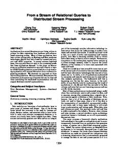
We use 4 data sets of IP flows collected on a large ISP network in a 10 minute interval during October 2005. We looked at aggregations according to IP source address (366K distinct values), IP destination address (517K distinct values), source port (55K distinct values), and destination port (57k distinct values). We also use three additional Web traffic datasets: WorldCup: Web server log from the 1998 World soccer championship, with 4021 distinct items. Dec-64: Web proxy traces that were recorded at Digital Equipment Corporation in 1996, with 497597 items. Lbl-100: 30 days of all wide-area TCP connections between the Lawrence Berkeley Laboratory (LBL) and the rest of the world, with 13783 distinct items. Figure 1 shows the top-k weights for these distributions that show an obvious Zipf-like form. 1

1

top-k weight

top-k weight

0.1

0.01

0.001

source port dest port source IP address dest IP address

0.0001 1

10

100

1000 k

10000

100000

0.1

worldcup lbl100 dec64

0.01 1e+06

1

IP flows

10

100

1000 k

10000

100000

1e+06

Web datasets

Figure 1: top-k weights for test distributions

3 Basic bounds for top-k sampling When estimating a proportion, we use the fraction of positive examples in the sample as our estimator. Using the notation we introduced earlier, we can use the interval from L(ˆ p, s, δ) to U (ˆ p, s, δ) as a 2δ confidence interval. It is also well understood how to obtain the number of samples needed for proportion estimation within some confidence and error bounds when the proportion is at least p. When estimating the top-k weight from samples, we would like to derive confidence intervals and also to determine the size of a fixed sample needed to answer a top-k query when the weight of the top-k set is at least p. 7

The natural top-k candidate is the set of k most sampled items. The natural estimator for the weight of the top-k set is the sampled weight of the sampled top-k items. This estimator, however, is inherently biased. The expectation of the sampled weight of the sample top-k is always at least as large and generally is larger than the weight of the top-k set. The bias depends on the number of samples and vanishes as the number of samples grows. It also depends on the distribution. To design estimation procedures or to obtain confidence intervals for a top-k estimate we have to account for both the standard error, as in proportion estimation, and for the bias.

3.1

Top-k versus proportion estimation

We show that top-1 estimation is at least as hard as estimating a proportion. Intuitively, we expect this to be the case. Estimating proportion is equivalent to estimating a single fixed item, whereas when we estimate the top-1 we have, in a sense, to bound more than one item. Lemma 5. Let A be an algorithm that approximates the top-1 weight in a distribution with confidence 1−δ. We can use A to derive an algorithm A′ for estimating a proportion. The accuracy of A′ when estimating a proportion p is no worse than the accuracy of A on a distribution with top-1 weight equals to p. Proof. An input to A′ is a set S ′ of s coin flips of a coin with bias p. Algorithm A′ translates S ′ to a sample S from a distribution D in which we have one item b of weight p and every other item has negligibly small weight. We generate S by replacing each positive sample in S ′ by a draw of b and every negative example in S ′ by a draw of a different element (a unique element per each negative example). Algorithm A′ applies A to S and returns the result. It is also not hard to see that the top-k problem is at least as hard as the top-1 problem. This is obvious for the stronger (per item) versions of the top-k problem but also holds for the approximate top-k weight problem. To see this, consider a stream of samples for a top-1 problem. Replace each sample of item i by a sample of an item labeled (i, x) where x is chosen uniformly from {0, . . . , k − 1}. This is equivalent to drawing from a distribution where each item is partitioned to k parts of the same weight. The top-k weight in this distribution is the same as the top-1 weight in the original distribution.

4 The Naive confidence interval Let Lk (fˆ, s, δ) be the smallest f such that there exists a distribution F , with top-k weight of f , such that when sampling S of size s we have P ROB{W k (S, F ) ≥ fˆ} ≥ δ. Similarly, let Uk (fˆ, s, δ) be the largest f such that there exists a distribution F with top-k weight of f such that when sampling S of size s, P ROB{W k (S, F ) ≤ fˆ} ≥ δ. Let S be a sample of s items from a distribution I and assume that fˆ = W k (S, I). By a proof similar to that of Lemma 1 one can show that Lemma 6. Uk (fˆ, s, δ) is a (1 − δ)-confidence upper bound on the top-k weight, and Lk (fˆ, s, δ) is a (1 − δ)confidence lower bound on the top-k weight. We define the Naive (1 − δ)-confidence interval to be [Lk (fˆ, s, δ/2), Uk (fˆ, s, δ/2)]. Note that since the (1 − δ/2)-confidence upper bound and the (1 − δ/2)-confidence lower bound are not symmetric we may be able to reduce the length of the interval by splitting the δ confidence asymmetrically between the upper and the lower bounds. That is, for every 0 < δ ′ < δ, [Lk (fˆ, s, δ ′ ), Uk (fˆ, s, δ − δ ′ )] is also a confidence interval that may be smaller than [Lk (fˆ, s, δ/2), Uk (fˆ, s, δ/2)].

8

4.1

Computing the Naive confidence interval

Our definitions do not provide an immediate way to compute the Naive confidence interval, since they require to consider all possible distributions. We now describe an algorithm to compute these bounds. We first consider the upper bound and show that we can use the (1 − δ)-confidence upper bound for a proportion as a (1 − δ)-confidence upper bound on the top-k weight. Lemma 7. Uk (fˆ, s, δ) ≤ U (fˆ, s, δ). Lemma 7 follows from the following lemma. Lemma 8. The distribution function of the sampled weight of the sampled top-k dominates that of the sampled weight of the top-k set. That is, for all α > 0, P rob{W k (S, I) ≥ α} ≥ P rob{w(S, Tk (I)) ≥ α} . In particular, E(W k (S, I)) ≥ W k (I) (the expectation of the sampled weight of the sampled top-k set is an upper bound on the actual top-k weight.) Proof. Observe that the sample weight of the sampled top-k is at least as large as the sampled weight of the actual top-k set (assume top-k set is unique using arbitrary tie breaking). Proof. [of Lemma 7] Let Uk (fˆ, s, δ) = f , and let F be a distribution with top-k weight f such that P ROB{W k (S, F ) ≤ fˆ} ≥ δ. By Lemma 8 we have that P rob{W k (S, I) ≤ fˆ} ≤ P rob{w(S, Tk (I)) ≤ fˆ} . Since the right hand side equals to the probability that in s tosses of a coin with success prob. f we get ≤ fˆs successes we get that the latter probability is at least δ. It follows that f ≤ U (fˆ, s, δ). We next consider how to obtain a lower bound on the top-k weight. The definition of Lk (fˆ, s, δ) was with respect to all distributions. The following Lemma restricts the set of distributions that we have to consider. We can then compute Lk (fˆ, s, δ) using simulations with the restricted set of distributions. Let I1 and I2 be two distributions. We say that I1 dominates I2 if for all i ≥ 1, W k (I1 ) ≥ W k (I2 ). The next lemma shows that if I1 dominates I2 then the distribution of the sampled weight of the sampled top-k of I1 dominates that of I2 . Lemma 9. If the distribution I1 dominates the distribution I2 then for any k ≥ 1, and number of samples s ≥ 1, the distribution function of the sampled weight of the sampled top-k in a sample of size s from I1 dominates the same distribution function with respect to I2 . That is, for any t, the probability that the sampled top-k in a sample from I1 has at least t samples is at least as large as the same probability with respect to I2 . Proof. We prove the claim for two distributions I1 and I2 that are identical except for two items b1 and b2 . In I2 the items b1 and b2 have weights w1 and w2 , respectively where w1 > w2 . In I1 the items b1 and b2 have weights w1 + ∆ and w2 − ∆, respectively for some ∆ ≥ 0. Clearly if the claim holds for I1 and I2 as above then it holds in general. This is true since given any two distributions I1 and I2 such that I1 dominates I2 we can find a sequence of distributions I2 = I 0 , I 1 , . . . , I ℓ = I1 where for every 0 ≤ j < ℓ, I2j+1 is obtained from I2j by shifting ∆ weight from a smaller item to a larger one. Consider a third distribution I3 that is identical to I1 and I2 with respect to all items other than b1 and b2 . The distribution I3 , similar to I1 , it has an item b1 with weight w1 , an item b2 of weight w2 − ∆ and an additional item b3 of weight ∆. 9

We sample s items from I2 by sampling s items from I3 and considering any sample of b2 or b3 as a sample of b2 . Similarly we sample s items from I1 by sampling s items from I3 and considering a sample from b2 as a sample of b2 and a sample of either b1 or b3 as a sample of b1 . Suppose we sample a set S of s items from I3 and map them as above to a sample S1 of s items from I1 and to a sample S2 of s items from I2 . We show that for every k and t, P rob{W k (S1 , I1 ) ≥ t} is not smaller than P rob{W k (S2 , I2 ) ≥ t}. Fix the number of samples of each item different of b1 , b2 , and b3 , fix the number of samples of b3 to be r, fix the number of samples of b1 and b2 together to be m, fix m/2 ≤ j ≤ m and assume that either b1 or b2 gets j our of the m samples. Consider only samples S of I3 that satisfy these conditions. We look at the probability space conditioned on these choices where the only freedom that we have left is which of b1 and b2 gets j samples (the other then gets m − j samples). We show that in this subspace, for every k and t, P rob{W k (S1 , I1 ) ≥ t} is not smaller than P rob{W k (S2 , I2 ) ≥ t}. Over this conditioned probability subspace, let Aj be the event where the number of samples of b1 is j and the number of samples of b2 is m − j, and let Am−j be the event where the number of samples of b1 is m − j and the number of samples of b2 is j. In Aj the maximum among the weights of b1 and b2 in S1 is max{j + r, m − j} = j + r, and the maximum among the weights of b1 and b2 in S2 is max{j, m − j + r} which is smaller than j + r. On the other hand, in Am−j the maximum among the weights of b1 and b2 in S1 is max{m−j +r, j}, and the maximum among the weights of b1 and b2 in S2 is max{m−j, j +r} = j +r. Consider the weight of the top-k set of S2 in Am−j , and the weight of the top-k set of S1 in Am−j . If both are at least t then they both are at least t in Aj , and both P rob{W k (S1 , I1 ) ≥ t} and P rob{W k (S2 , I2 ) ≥ t} equal 1. However it could be that in Am−j the weight of the top-k set of S2 is larger than t but the weight of the top-k set in S1 is smaller than t. However if this is indeed the case in Am−j , then in Aj the weight of the top-k set of S1 is larger than t but the weight of the top-k set in S2 is smaller than t. Let a = w1 /(w1 + w2 − ∆). Since µ ¶ µ ¶ m m P rob{Aj } = aj (1 − a)m−j ≥ (1 − a)j (a)m−j = P rob{Am−j } , j j it follows that P rob{W k (S1 , I1 ) ≥ t} is not smaller than P rob{W k (S2 , I2 ) ≥ t}. Lemma 9 identifies the family of “worst-case” distributions among all distributions that have top-k weight equal to f . That is, for any threshold t and for any k, one of the distributions in this family maximizes the probability that the sampled weight of the sampled top-k exceeds t. Therefore, to find Lk (fˆ, s, δ), it is enough to consider the more restricted set of most-dominant distributions. The most-dominant distribution is determined once we fix both the weight f of the top-k, and the weight 0 < ℓ ≤ f /k of the kth largest item. The top-1 item in this distribution has weight f − (k − 1)ℓ, the next k − 1 heaviest items have weight ℓ, next there are ⌊(1 − f )/ℓ⌋ items of weight ℓ and then possibly another item of weight 1 − f − ℓ⌊(1 − f )/ℓ⌋. Example is provided in Figure 3. Fix the weight f of the top-k. Let Gℓ be the most dominant distribution with value ℓ for the kth largest item. We can use simulations to determine the threshold value tℓ so that with probability δ, the sampled weight of the sampled top-k in s samples from Gℓ is at least tℓ . Let fm = maxℓ tℓ . Clearly fm decreases with f . The value Lk (fˆ, s, δ) is the largest f such that fm ≤ fˆ. This mapping from the observed value fˆ to the lower bound f can be computed once and stored in a table, or can be produced on the fly as needed. Note that for the top-1 problem, there exists a single “worst-case” most-dominant distribution, this distribution has ⌊1/f ⌋ items of weight f and possibly an additional item of weight 1 − f ⌊1/f ⌋.

10

4.2

Bounding the weight of the top-k set

We now consider the problem of bounding the (real) weight of the sampled top-k set. We define a (1 − δ)confidence lower bound L′ (fˆ, s, δ) on the actual weight of top-k set: L′ (fˆ, s, δ) is the minimum ℓ such that there exists a distribution I with the following property. When sampling a set S of size s from I then P ROB{(W k (S, I) ≥ fˆ) ∧ (w(Tk (S, I)) ≤ ℓ)} ≥ δ. It is easy to see that L′k (fˆ, s, δ) ≤ Lk (fˆ, s, δ) since if we restrict the distributions I that we consider when defining L′k (fˆ, s, δ) to those with top-k weight at most ℓ we obtain Lk (fˆ, s, δ). Lemma 10. L1 (fˆ, s, δ) is a (1 − δ)-confidence lower bound on the weight of the sampled top-1 item. Proof. Consider a distribution I with top-1 item of weight greater then ℓ. If P ROB{(W 1 (S, I) ≥ fˆ) ∧ (w(T1 (S, I)) ≤ ℓ)} ≥ δ then P ROB{(W 1 (S, I ′ ) ≥ fˆ) ∧ (w(T1 (S, I ′ )) ≤ ℓ)} ≥ δ where I ′ is obtained from I by splitting all items of weight larger then ℓ into small items. For k > 1 we conjecture the following: Conjecture 11. Lk (fˆ, s, δ) is a (1 − δ)-confidence lower bound on the weight of the sampled top-k set. To prove the conjecture we need to show that L′k (fˆ, s, δ) = Lk (f, s, δ), that is, there is distribution that minimize ℓ that has top-k weight that is at most ℓ. Our experiments support the conjecture as we always observed that the actual weight of the top-k weight lies inside the confidence interval.

4.3

Asymptotics of the Naive estimator

For a given distribution I, and a given ǫ and δ, consider the smallest number of samples m(I) such that the sampled weight of the sampled top-1 item in m(I) samples is in the interval (1 ± ǫ)W 1 (I) with confidence 1 − δ. The maximum m(I) over all distributions I with top-1 item of weight f is the smallest number of samples that suffices to answer a top-1 query for a specified δ and ǫ, when I has top-1 weight at least f . The distribution I with top-1 item of weight f that maximizes m(I) has about 1/f items of weight f . To estimate W 1 (I) to within (1 ± ǫ), each of these f1 items has to be estimated to within (1 ± ǫ) with confidence 1 − f δ. Using multiplicative Chernoff bounds we obtain that the number of samples needed is O(f −1 ǫ−2 (ln δ −1 + ln f −1 )), which is super linear in f −1 . One can contrast this with the number of samples needed to estimate a proportion of value at least f , for a given ǫ, δ, and f . From Chernoff bounds we have O(f −1 ǫ−2 ln δ −1 ), which is linear in f −1 . The Naive bound is derived under “worst-case” assumptions on the distribution, and therefore the asymptotic of O(f −1 ǫ−2 (ln δ −1 + ln f −1 )) applies to it. A distribution in which all items other than the top-1 are tiny behaves like a proportion and for such distributions we obtain a good estimate of the top-1 weight after O(f −1 ǫ−2 ln δ −1 ) samples. Estimating the top-k weight in a Zipf-like distributions, that arise in natural settings, is similar to estimating proportion as the distribution becomes more skewed. This point is demonstrated in Figure 2. The figure shows sampling from a distribution with top-1 item of weight 0.05. It shows the sampled weight of the sampled top-1 item on a uniform distribution where there are 20 items of weight 0.05 each. It also shows the sampled weight of a sampled top-1 item in a distribution where there is a single item of weight 0.05 and all other items have infinitesimally small weight. The averaging of the expected sampled weight of the sampled top-1 over 1000 runs illustrates the bias of the estimator on the two distributions. Evidently, the bias quickly vanishes on the second distribution but is significant for the uniform distribution. The Naive confidence bound accounts for this maximum possible bias, so even on this simple distribution, after 10, 000 samples we are only able to guarantee a 5% error bars. The figure shows a similar situation when we measure the sampled weight of the top-5 items in a distribution with 5 items of weight 0.05 each and all other items infinitesimally small. The convergence is 11

similar to that of estimating a proportion of 0.25; When there are 20 items of weight 0.05, convergence is much slower and there is a significant bias. 0.1 0.08 0.06 0.04

0.06

0.04

0.02

0.02

0 1

0.4

2 3 4 5 6 7 8 number of thousands of samples

9

0

10

1

0.4

top-5 uniform top-5 proportion-like top-5 weight

0.35

2

3 4 5 6 7 8 number of thousands of samples

9

10

9

10

top-5 unifrom top-5 proportion-like top-5 weight

0.35 0.3 weight

0.3 weight

top-1 uniform top-1 proportion-like top-1 weight

0.08

weight

weight

0.1

top-1 uniform top-1 proportion-like top-1 weight

0.25

0.25

0.2

0.2

0.15

0.15

0.1

0.1 0

1

2 3 4 5 6 7 8 number of thousands of samples

9

10

0

A single set of samples

1

2 3 4 5 6 7 8 number of thousands of samples

Average of 1000 sets of samples

Figure 2: Convergence of the Naive top-k estimator. The top figures are for top-1 item of weight 0.05. The bottom figures for the top-5 items of weight 0.25. The curve “top-1 uniform” shows the sample weight of the sampled top-1 item in a uniform distribution. The curve “top-1 proportion-like” shows the sample weight of the sampled top-1 item from a distribution with a single item of weight 0.05 and all the rest infinitesimally small. The plots for top-5 are annotated similarly. These arguments indicate that the Naive estimator gives a pessimistic lower bounds that also exhibit worse asymptotics than what we can hope to obtain for some natural distributions. We therefore devise and evaluate procedures to derive tighter lower bounds by exploiting more information on the distribution.

5 Using a cumulative upper bound The derivation of the CUB resembles that of the Naive bound. We use the same upper bound and the difference is in the computation of the lower bound. As with the Naive bound, we look for the distribution with the smallest top-k weight that is at least δ likely to produce the sampled top-k weight that we observe. The difference is that we do not use the sampled top-k weight only, but extract more information from the sample to further restrict the set of distributions we have to consider, thereby tightening the bound. The bound is derived in two steps where we split the confidence, δ, into δ ′ ≤ δ for the first step, and δ − δ ′ for the second step. 12

1. Cumulative upper bound (CUB) derivation: We obtain (1 − δ ′ )-confidence cumulative upper bound {K(i)} = K(1), K(2), . . . such that K(i) is an upper bound on W i (I) for all i ≥ 1 with probability (1 − δ ′ ). 2. Lower bound derivation: Let fˆ = W k (S, I). We derive a (1 − (δ − δ ′ ))-confidence lower bound ′ ˆ Lcub k ({K(i)}, f , s, δ −δ ) which is defined as follows. We consider all distributions that are consistent with the CUB {K(i)}: that is distributions J such that W i (J) ≤ K(i) for all (i ≥ 1). Among these distributions we look for the distribution J with smallest top-k weight W k (J) that is at least (δ − δ ′ ) likely to have a sampled top-k weight of at least fˆ. The lower bound is then set to W k (J). Correctness follows since for any distribution the probability that the cumulative upper bound obtained for it fails (even for one value) is at most δ ′ . If the distribution obeys the cumulative upper bound derived for it in the first stage then the probability that the lower bound derived in the second step is incorrect is at most (δ − δ ′ ). Therefore, for any distribution, the probability that it does not lie in its confidence interval is at most δ. A formal argument for correctness of the second stage is analogous to the one of Lemma 1, Lemma 2, and Lemma 6. Note also that if K(i) = 1 for all i ≥ 1 then the CUB bound degenerates to the Naive bound. In ˆ ˆ particular Lcub k ({1, 1, 1, 1, 1...}, f , s, δ) = Lk (f , s, δ). We obtain the upper bounds K(i) either by Lemma 3 or by lemma 4. We have that fˆ = W k (S, I). W i (S,I) Using Lemma 3 we let q be the value such that q(1 − R(q, s, δ)) = fˆ and let K(i) = G(i) = 1−R(q,s,δ) for i ≥ k. We use G(i) = 1 for i < k. Alternatively, we use Lemma 4, set q to be the value such that W i (S,I) q(1 − R+ (q, s, δ)) = fˆ and let K(i) = G+ (i) = 1−R + (q,s,δ) for all i ≥ 1. Recall that we precompute + R(q, s, δ) and R (q, s, δ) for many possible values of q. ˆ We compute (1 − δ)-confidence lower bound, Lcub k ({K(i)}, f , s, δ), by considering most dominant distribution as follows. We apply Lemma 9 in a way similar to its usage in Section 4.1 for the Naive bound. We obtain that the most dominant distributions that satisfy the {K(i)} upper bounds is determined once we fix the top-k weight f and the weight ℓ ≤ f /k of the kth heaviest item. For i > k, the weight of the ith item is as large as possible given that it is no larger than the (i − 1)th item and that the sum of the top-i items is at most K(i). If K(1) = K(2) = . . . = K(k − 1) = 1, then the k-heaviest items are as in the naive bounds: the top-1 weight is f − (k − 1)ℓ and the next k − 1 heaviest items have weight ℓ. Otherwise, let 1 ≤ j ≤ k be the minimum such that K(j) + (k − j)ℓ ≥ f . The most dominant distribution is such that item ℓ for ℓ < j has weight K(i) − K(i − 1) with (K(0) = 0); items j + 1, . . . k have weight ℓ; and the jth item has weight f − K(j − 1) − (k − j)ℓ. Figure 3 shows most dominant distributions for k = 100 with top-k weight equal to 0.4 that are constructed subject to CUB constraints K(i) for i ≥ 100 and K(1) = . . . = K(99) = 1. The dotted lines show the most dominant distributions without the CUB constraints. The figure helps visualize the benefit of the CUB. The CUB constraints reduce the size and the number of larger non top-k items and by doing so reduces the bias of the top-k estimator (the sampled weight of the sample top-k). We use simulations on these most-dominant distributions to determine the probability that the sampled weight of the sampled top-k matches or exceeds the observed one. Since the CUB has many parameters ({K(i)} for i ≥ 1), we can not use a precomputed table for the cub ˆ ˆ lower bound Lcub k ({K(i)}, f , s, δ) as we can do for the naive bound Lk (f , s, δ). Therefore the CUB bounds are more computationally intensive than the Naive bound. The confidence interval that we obtain applies to the weight W k (I) of the top-k set. Using an argument similar to the one we used in Lemma 10, for k = 1, the confidence interval also applies to the actual weight of the sampled top-1 set. We conjecture that it also applies to the actual weight of the sampled top-k set when k > 1 (see Conjecture 11). 13

Cumulative item weight

1

0.8

0.6

0.4 l=0.004 0.2 l=0.002 l=0.0001

0 0

200

400

600 items

800

1000

1200

Figure 3: Most dominant distributions for k = 100 and top-k weight 0.4. These distributions are for ℓ = 0.004 (Uniform), ℓ = 0.002, and ℓ = 0.0001. We also show the distributions subject to CUB K(i) for i ≥ 100. The distributions with and without the CUB are identical for i ≤ 100. With CUB the straight lines for ℓ = 0.004 and ℓ = 0.002 start bending at some i > 100 to obey the CUB. Without the CUB they continue according to the lightly shaded straight lines. The distribution with ℓ = 0.0001 is not affected by the CUB.

14

The CUB method is based on performing simulations based on statistics derived from the sample and in this sense it is related to statistical bootstrap method [ET93].

6 Cross validation methods In this chapter we borrow some concepts from machine learning and use the method of cross validation to obtain confidence bounds. Intuitively, the methods we present in this section are based on the following lemma. Lemma 12. Let S ′ and S ′′ be two subsets of the sample S such that S ′ ∩ S ′′ = ∅. Let T be the top-k subset in S. Then the weight of T in S ′′ is unbiased estimate of the real weight, w(T ), of T . ′′

Proof. In fact, w(S , T ) is a random variable counting the fraction of successes when we toss a coin of bias w(T ), |S ′′ | times. We start with a simple split-sample validation method. This method gives a top-k candidate and a lower bound on its actual weight. Then we generalize this method and describe the f -fold cross validation method and the leave-mℓ -out cross validation method that partition the sample to more than two parts. The expectation of all these estimators is equal to the expectation of the actual weight of a sampled top-k set obtained in a sample of size equal to that of the learning part. Since the actual weight of any top-k set is smaller than W k (I) these estimators are biased down and their expectation is smaller than W k (I). For a larger learning set, this expectation is higher and closer to W k (I), and therefore may give tighter bound. On the other hand, the variance of the estimate depends on the size of the testing set. We study these tradeoffs. Since these estimators are biased down we show how to use them to obtain the lower end of a confidence interval. We can obtain the upper end as we did for the Naive and the CUB methods. We also study a technique to upper bound the difference between the weight of our set to that of the actual top-k set. That is, upper bound the potential increase in weight by exchanging items in our candidate set with items outside it. We combine this technique with the split-sample method.

6.1

Split-sample (hold out) validation

We denote the learning part of S by Su and the testing part by Sℓ , and their sizes by mu and mℓ respectively. We used mu = mℓ = s/2, where |S| = s, but other partitions are possible. The sampled top-k set in the learning sample, Ik,u = Tk (Su , I), is our top-k candidate, and its sampled weight w(Sℓ , Ik,u ) in the testing sample is the split-sample estimator for the top-k weight. By Lemma 12, for every possible Ik,u , the expectation of the sampled weight of Ik,u in Sℓ equals to the actual weight of Ik,u . Since w(Ik,u ) ≤ W k (I), the expectation of w(Sℓ , Ik,u ) is a lower bound on W k (I). We obtain confidence bounds based on this estimator as follows. For an upper bound we use U (δ) = U (W k (S, I), m, δ) as in the previous methods. Since the variance of this estimator is no larger than the variance of a proportion with mℓ flips we use L(δ) = L(w(Sℓ , Ik,u ), mℓ , δ) as our lower bound. For both upper and lower bounds we take [L( 2δ ), U ( 2δ )] as our (1 − δ) - confidence interval. Note that our estimate is valid not only for the top-k weight but also for the actual weight of the set Ik,u .

6.2

2-fold cross validation

In 2-fold cross validation we split the sample S into two equal parts Su and Sℓ . Let Ik,u and Ik,ℓ be the sampled top-k sets in Su and Sℓ , respectively. The 2-fold estimator is (w(Sℓ , Ik,u ) + w(Su , Ik,ℓ ))/2. This estimator is an average of two estimators X = w(Sℓ , Ik,u ) and Y = w(Su , Ik,ℓ ). The expectation of each 15

of these two estimators equals to the average weight of a top-k set in a sample of size s/2. So by linearity of expectation this is also the expectation of the 2-fold estimator. Clearly by Lemma 12 the expectation of this estimator is at most W k (I). We turn this estimator into a confidence interval in a way similar to what we did for the split sample estimator. But for the lower bound we use L(δ) = L((w(Sℓ , Ik,u ) + w(Su , Ik,ℓ ))/2, s/2, δ). To see that this is a (1 − δ)-confidence lower bound let X = w(Sℓ , Ik,u ) and Y = w(Su , Ik,ℓ ). Note that in general we have µ ¶ X +Y V ar(X) + V ar(Y ) + 2Cov(X, Y ) V ar , (2) = 2 4 where Cov(X, Y ) is the covariance of X and Y . Since 2Cov(X, Y ) = 2E(XY ) − 2E(X)E(Y ) ≤ E(X 2 ) + E(Y 2 ) − 2E(X)E(Y ) , and in our case E(X) = E(Y ), we have ¡ X+Ythat ¢ 2Cov(X, Y ) ≤ V ar(X) + V ar(Y ). Furthermore since V ar(X) = V ar(Y ) we have that V ar ≤ V ar(X). This implies that a lower bound for a proportion 2 with s/2 flips applies. Although in our case X and Y ¡are not¢ independent we expect them to be weakly correlated, in which case Cov(X, Y ) is small and V ar X+Y is close to V ar(X)/2 as if X and Y were 2 independent. Our lower bound is worst-case and does not take this observation into account. Our experiments indicate that the following conjecture analogous to Conjecture 11 may be true. Conjecture 13. L(δ) is a (1 − δ)-confidence lower bound on the weight of the set Tk (S, I).

6.3

R-fold cross validation

In general by partitioning the samples into r equal parts we get the r-fold cross validation estimator. For each part, we compute the sampled top-k set in the union of the other r − 1 parts (the learning set). Then we compute the weight of this set in the held-out part (the testing set). Let Xj , 1 ≤ j ≤ r be a random variable that denotes this weight when the j-th part is held out. The following lemma follows from Lemma 12. Lemma 14. For any j, E(Xj ) ≤ W k (I). The r-fold estimator is

6.4

Pr

j=1

Xj

r

.

Leave-out cross validation

Leave-mℓ -out cross validation is a “smoothed” version of r-fold cross validation. Consider some fixed k ≤ mu ≤ m − 1. The estimator Jmu is the average, over all subsets Su ⊂ S of size |Su | = mu , of the sampled weight in Sℓ = S \ Su of the sampled top-k subset in Su . When there are multiple items with kth largest number of samples we average the sampled weight in Sℓ of all possible top-k sets in Su . The following lemma follows from Lemma 12 and the linearity of expectation. Lemma 15. For all mu , E(Jmu ) ≤ W k (I). Let mℓ = |Sℓ | and assume

|S| mℓ

is an integer, then we expect this leave out estimator Jmu to have smaller

|S| |S| . As for r-fold with r = m , the expectation of the estimator variance than of an r-fold estimator with r = m ℓ ℓ Jmu is equal to the expectation of the actual weight of the sampled top-k set in a sample of size mu .

16

6.5

Computing leave-out estimators

The leave-out estimator is defined as an average over all possible subsets, so its direct computation can be prohibitive. In this section we develop a method to estimate the leave-out estimator. We defined Jmu as an average over all subsets Su ⊂ S of size |Su | = mu , of the sampled weight in Sℓ = S \ Su of the sampled top-k subset in Su . Alternatively, we can sum for each occurrence x of an item i in S, the number of subsets Su of S \ {x} where i is in the top-k set of Su , and then divide this by the total number of subsets of size mu . Let Pk (i, m, S) be the number of subsets S ′ of size m, of a multiset S where i is in the top-k subset of S ′ . To carefully account for subsets S ′ in which the top-k set is not uniquely defined, a more precise definition of Pk (i, m, S) is as follows. We consider every subset S ′ of size m of S. Let ℓ be the number of occurrences of the kth most frequent item in S ′ . If the frequency of i in S ′ is larger than ℓ then S ′ contributes 1 to Pk (i, m, S). If the frequency of i in S ′ is smaller than ℓ then S ′ contributes 0 to Pk (i, m, S). Otherwise, let b be the total number of items with frequency equal to ℓ, and let c be the number of such items in the top-k set of S ′ . The contribution of S ′ to Pk (i, m, S) is c/b. The following lemma gives an equivalent formulation of Jmu . Lemma 16. Let i be the the ith most frequent item in S and let ai be the number of occurrences of i in S. Let xi be one among the ai occurrences of i in S. Then P ai Pk (i, mu , S \ {xi }) Jmu = i . ¡ |S| ¢ mu

Pk (i,mu ,S\{xi })

by sampling random subsets of size mu from S \ {xi }, |S| ) (m u compute the contribution to Pk (i, mu , S \ {xi }) of each subset, and divide by the number of subsets we sampled. To make this computation more efficient we sample subsets of size mu + 1 from S. For each such subset S ′ , and for each occurrence, x, of an item i in S ′ , we use S ′ \ {x} as a random sample from S \ {x} and use it in the estimation of Pk (i,mu|S|,S\{xi }) . (mu ) For each item i we can estimate

Leave-1-out. The leave-1-out and the s-fold estimators (where s = |S|) are the same. We can compute this estimator efficiently from the counts of items in the sample. Consider a sample S and let a1 ≥ a2 ≥ a3 · · · be the counts of the items in S. Let tk+1 ≥ 1 be the number of items with frequency equal to ak+1 . Let n (0 ≤ n ≤ tk+1 − 1) be the number of items with frequency ak+1 in the sampled top-k set. The estimate is

Js−1

 µ ¶ 1  = s

X

i|ai >ak+1 +1

ai +

µ

n+1 tk+1 + 1

¶

X

i|ai =ak+1 +1



ai  .

The first terms account for the contribution of items that definitely remain in the modified top-k set after “loosing” the leave-out sample. This includes all items that their count in the sample is larger than ak+1 + 1. The second term accounts for items that are “partially” in the top-k set after loosing the leaveout sample. By partially we mean that there are more items with that frequency than spots for them in the new top-k set. The hypothesis testing literature indicates that leave-1-out cross validation performs well but has the disadvantage of being computationally intensive. In our setting, the computation of the estimator is immediate from the sampled frequencies. This estimator has a learning set of maximal size, s − 1, and therefore its expectation is closest to the top-k weight among all the cross validation estimators. 17

6.6

Bounding the variance.

The choice of the particular cross validation estimator, selecting r for the r-fold estimators or mu for the leave-out estimators reflects the following tradeoffs. The expectation of these estimators is the expectation of the actual weight of the sampled top-k set in a sample of the size of the learning set. This expectation is non-decreasing with the number of samples and gets closer to W k (I) with more samples in the learning set. Therefore, it is beneficial to use larger learning sets (small r, or large mu ). In the extreme, the leave-1-out estimator is the one that maximizes the expectation of the estimator. However, smaller size test sets and dependencies between learning sets can increase the variance of the estimator. The effect of that on the derived lower bound depends on both the actual variance and on how tightly we can bound this variance. In our evaluation, we consider both the empirical performance of these estimators and the rigorous confidence intervals we can derive for them. As we did with the 2-fold estimator, we can apply proportion lower bounds to any of the cross validation estimators to obtain the lower end of a confidence interval as follows. Since the variance of the estimator is not larger than the variance of a Binomial random variable with mℓ = s − mu³(or P s/r) independent ´ r

Xj

j=1 samples we apply the proportion lower bound to it. For the r-fold method we have L , rs , δ as our r 1 − δ-confidence lower bound, and for the leave-mℓ -out estimator we obtain L (Jmu , mℓ , δ). This method is pessimistic for two reasons. The first is the application of a proportion bound to a biased quantity. The second reason is that the calculation assumes a binomial distribution with mℓ or s/r independent trials, and therefore does not account for the benefit of the cross validation averaging over multiple splits into learning and test subsets. This effect becomes worse for larger values of r. (See the discussion in Section 6.2.) In the experimental evaluation, we consider both the empirical performance of the estimators (in terms of expectation and the average squared and absolute error), and the quality of the confidence intervals. For confidence intervals, we use two approaches to derive lower bounds: The first is the pessimistic rigorous approach. The second is a heuristic that “treats” the estimate as a binomial with s independent trials and applies a proportion L(Z, s, δ) lower bound, where Z is the value of the estimator. We refer to this heuristic as r-fold with s and carefully evaluate its empirical correctness.

6.7

Weight difference to the top-k weight

We next consider the goal of obtaining a (1 − δ)-confidence upper bound on the difference W k (I) − w(Ik,u ) between the weight of our output set Ik,u to that of the true top-k set. A more refined question is “by how much can we possibly increase the weight of our set by exchanging items from Ik,u with items that are in I \ Ik,u ?” It is a different question than bounding the weight of the set. For example, in some cases we can say that “we are 95% certain that our set is the (exact) top-k set”, which is something we can not conclude from confidence bounds on the weight. We use the basic split-sample validation approach, where the top-k candidate set, Ik,u , is derived from the learning sample Su . The testing sample Sℓ is then used to bound the amount by which we can increase the weight of the set Ik,u by exchanging a set of items from Ik,u with a set of items of the same cardinality from I \ Ik,u . Let Cj = C(W j (Sℓ , I \ Ik,u ), mℓ , W j (Sℓ , Ik,u ), mℓ , δ). Recall that C() was define in Section 2. It is a (1 − δ)-confidence upper bound on the difference of two proportions. To obtain Cj we apply it as if we observe W j (Sℓ , I \ Ik,u ) positive examples in mℓ draws of one proportion and W j (Sℓ , Ik,u ) positive examples of the other in mℓ draws. Lemma 17. max1≤j≤k Cj is a (1 − δ)-confidence upper bound on the amount by which we can increase the weight of the set Ik,u by exchanging items. (Hence, it is also a (1 − δ)-confidence upper bound on the 18

difference W k (I) − w(Ik,u ).) Proof. The maximal amount by which we can increase the weight of Ik,u by exchanging items is equal to max W j (I \ Ik,u ) − W j (Ik,u ) .

1≤j≤k

It follows that if Cj is a (1 − δ)-confidence upper bound on the difference W j (I \ Ik,u ) − W j (Ik,u ), then max1≤j≤k Cj is a (1−δ)-confidence upper bound on the maximum increase (and therefore on the difference W k (I) − w(Ik,u ).) It remains to show that Cj is a (1 − δ)-confidence upper bound on W j (I \ Ik,u ) − W j (Ik,u ). We use the samples Sℓ to obtain upper bound on the weight of the top-j elements in I \ Ik,u , and a lower bound on the weight of the bottom-j elements in Ik,u . Let Jj = Tj (I \ Ik,u ) be the real top-j set in I \ Ik,u . Let Hj = Bj (Ik,u ) be the real bottom-j set in Ik,u . Clearly W j (I \ Ik,u ) − W j (Ik,u ) = w(Jj ) − w(Hj ). The value w(Sℓ , Jj ) is equivalent to the fraction of positive examples in mℓ tosses of a proportion w(Jj ). Similarly, the value w(Sℓ , Hj ) is equivalent to the fraction of positive examples in mℓ tosses of a proportion w(Hj ). Since W j (Sℓ , I \ Ik,u ) ≥ w(Sℓ , Jj ) and W j (Sℓ , Ik,u ) ≤ w(Sℓ , Hj ) we obtain that W j (Sℓ , I \ Ik,u ) − W j (Sℓ , Ik,u ) ≥ w(Sℓ , Jj ) − w(Sℓ , Hj ) . Since Cj is an upper bound (with probability 1 − δ) on the difference of the proportions, assuming the outcomes from drawing the proportions are W j (Sℓ , I \ Ik,u ) and W j (Sℓ , Ik,u ), then it is clearly an upper bound with probability 1 − δ on w(Jj ) − w(Bj ) as required.

7 Evaluation Results The algorithms were evaluated on all data sets, for top-100 and top-1, and confidence levels δ = 0.1 and δ = 0.01. In the evaluation we consider the tightness of the estimates and confidence intervals. For the heuristic r-fold with s lower bounds we also consider correctness.

7.1

Quality of different estimators

We empirically evaluated the expectation, average square error, and average absolute error of the (positively biased) sampled weight of the sampled top-k items, and the negatively-biased split-sample, 2-fold, 10-fold, and s-fold estimators. We also consider two combined estimators: the average of the sampled weight of the sampled top-k items and the s-fold estimator (s-fold+upper) and the average of the sampled weight of the sampled top-k items and the 2-fold estimator (2-fold+upper). The expectation of these estimators shows their bias, the square and absolute error reflect both the bias and the variance of these estimators. The results for three datasets are shown in Figures 4 and 5. We only show the average absolute error, the average square error behaves similarly. The figures show that the bias decreases with r for the r-fold estimators. The absolute error and variance measures vary: 2-fold is always at least as good as split-sample and on some datasets it has considerably smaller variance. In most cases, the s-fold and 10-fold estimators have smaller variance than the 2-fold estimator. The sampled weight of the sampled top-k items is often worse or comparable to the s-fold estimator. The combined estimators perform very well and in most cases they had the smallest error and bias.

19

destIP k=100 average estimates

destIP k=100 average abs error 0.1

0.1

sample-weight sample-top-100 true-weight sample-top-100 split-sample 2-fold 10-fold s-fold 2-fold+upper s-fold+upper

weight

0.01 0.01 top-100 weight sample-weight sample-top-100 true-weight sample-top-100 split-sample 2-fold 10-fold s-fold 2-fold+upper s-fold+upper

0.001 1000

10000 samples

0.001

100000

0

5000 10000 15000 20000 25000 30000 35000 40000 45000 50000 samples

destIP k=1 average estimates

destIP k=1 average abs error

0.0025

0.002

weight

0.0015

top-1 weight sample-weight sample-top-1 true-weight sample-top-1 split-sample 2-fold 10-fold s-fold 2-fold+upper s-fold+upper

0.001

sample-weight sample-top-1 true-weight sample-top-1 split-sample 2-fold 10-fold s-fold 2-fold+upper s-fold+upper

0.001

0.0005 0.0001 0 1000

10000

100000

1000

samples

10000 samples

Figure 4: Average value (left) and corresponding average absolute error (right) of top-k estimators (averaged over 500 runs) for destination ports.

20

100000

srcIP k=100 average estimates

srcIP k=100 average abs error 0.1

weight

0.1 0.01 top-100 weight sample-weight sample-top-100 true-weight sample-top-100 split-sample 2-fold 10-fold s-fold 2-fold+upper s-fold+upper 1000

10000 samples

0.001 1000

100000

worldcup k=100 average estimates

10000 samples

100000

worldcup k=100 average abs error

0.64

0.1

0.62 0.6 0.58 weight

sample-weight sample-top-100 true-weight sample-top-100 split-sample 2-fold 10-fold s-fold 2-fold+upper s-fold+upper

0.56

sample-weight sample-top-100 true-weight sample-top-100 split-sample 2-fold 10-fold s-fold 2-fold+upper s-fold+upper

0.01

0.54 0.52 0.5 0.48 1000

top-100 weight sample-weight sample-top-100 true-weight sample-top-100 split-sample 2-fold 10-fold s-fold 2-fold+upper s-fold+upper 10000 samples

0.001 1000

100000

10000 samples

Figure 5: Average value (left) and corresponding average absolute error (right) of top-k estimators (averaged over 500 runs) for the source ports and the WorldCup data sets.

21

100000

7.2

Confidence intervals

We compared the Naive bound, the CUB bound, the split-sample and 2-fold bounds (with s/2 proportion correction), and the 10-fold bound (with s/10 proportion correction). The split-sample bound is similar to the 2-fold bound, and therefore not shown in the plots. Figure 6 shows averaged (1 − δ)-confidence upper and lower bounds for these methods. The upper bound is the same for all methods but the lower bound varies. We precomputed, using multiple simulation runs, tables for the (1 − δ)-confidence bounds U (ˆ p, s, δ), L(ˆ p, s, δ) (for proportions, see Section 2.2), and Lk (fˆ, s, δ) (for the Naive lower bound, see Section 4.1). The tables of Lk (fˆ, s, δ) were generated using a simulations with the families of most dominant distributions. We used the table of U (ˆ p, s, δ) to derive the upper bound, and the table of L(ˆ p, s, δ) to derive the lower bounds for the cross validation methods. We used the table of Lk (fˆ, s, δ) to derive the Naive lower bound. The precomputation of this table made the implementation of the Naive method very efficient. The implementation of the CUB method involved constructing and running simulations on families of mostdominant distributions in each run of the algorithms. For the CUB method, these families depend on the cumulative upper bounds obtained, so we could not use precomputed tables. As a result, the CUB method is considerably more computation intensive. We evaluated two variants of the CUB. The first one (denoted CUB in Figure 6) derives K(i) only for i ≥ k (K(1) = . . . = K(k − 1) = 1), using the method in Lemma 3. The second one (denoted CUB+ in Figure 6) uses a cumulative+ bound of Lemma 4 and thereby derives K(i) for all i ≥ 1. For a given confidence level, the bounds K(i) obtained by CUB+ are tighter for (i < k) but weaker for i ≥ k than the bounds obtained by CUB. There is a difference between CUB and CUB+ only for k > 1. The results for selected datasets and parameters (k and δ) are provided in Figure 6. The figures also show the top-k weight W k (I), the sampled weight of the sampled top-k set (that has expectation at least W k (I) and gets closer to W k (I) as the number of samples grows) the actual weight of the sampled top-k set (that has expectation at most W k (I) and also gets closer to W k (I) as the number of samples grows). The Naive lower bound is almost always the lowest (least tight) bound and is outperformed by the CUB and 2-fold bounds. The 10-fold bound is sometimes below Naive, because of the pessimistic s/10 proportion adjustment. In some cases, the Naive bound was tighter than the 2-fold bound. This can happen on distributions that are closer to the “most dominant distributions” on which the Naive bound is tight and the 2-fold method, that utilizes half the samples, is not. On our datasets, we observed that Naive is tighter on distributions where the top-k weight is most of the total weight. The CUB bound was tighter than the 2-fold bound on more distributions, but there were also many distributions where the 2-fold bound was tighter. The CUB+ bounds were slightly tighter than the CUB bounds. Observed error-rates for top-k weight. We considered the observed error rates of the (1 − δ)-confidence upper bounds and the (1 − δ)-confidence lower bounds obtained via rigorous methods (Naive, CUB, 2-fold with s/2 correction and 10-fold with s/10 correction). The observed error rate is the fraction of runs in which the lower bound was higher (or the upper bound was lower) than the top-k weight. Tables 1, 2, and 3 show the error rates for the upper bound and for the Naive and CUB lower bounds. The results are aggregated across different numbers of samples, for each dataset and k. When the number of experiments grows to infinity the error rate should be smaller than δ. For most instances (an instance is specified by the dataset, k, δ, method, and number of samples), the error rate was well below δ. This was the case since our worst case bounds are pessimistic. Observed error-rates for top-k set. We also considered the error rates of the (1 − δ)-confidence lower bounds with respect to the “top-k set” metric, that is the fraction of runs in which the actual weight of the

22

destIP k=100 delta=0.01 confidence bounds

destIP k=1 delta=0.01 confidence bounds

1

0.01

0.1

0.001

0.01

0.0001

0.001 0.0001 1e-05 1e-06 1000

1e-05

upper del=0.01 sample-weight sample-top-k top-k weight true-weight sample-top-k CUB lower del=0.01 CUB+ lower del=0.01 2-fold lower del=0.01 10-fold lower del=0.01 Naive lower del=0.01 10000

1e-06 1e-07 1e-08 1000

100000

srcport k=100 delta=0.01 confidence bounds 0.035

0.7

0.03

0.65

0.025

0.6

0.5 0.45 0.4 1000

0.02 upper del=0.01 sample-weight sample-top-k top-k weight true-weight sample-top-k CUB lower del=0.01 CUB+ lower del=0.01 2-fold lower del=0.01 10-fold lower del=0.01 Naive lower del=0.01 10000

10000

100000

worldcup k=1 delta=0.01 confidence bounds

0.75

0.55

upper del=0.01 sample-weight sample-top-k top-k weight true-weight sample-top-k CUB lower del=0.01 2-fold lower del=0.01 10-fold lower del=0.01 Naive lower del=0.01

upper del=0.01 sample-weight sample-top-k top-k weight true-weight sample-top-k CUB lower del=0.01 2-fold lower del=0.01 10-fold lower del=0.01 Naive lower del=0.01

0.015 0.01 0.005 100000

0 1000

srcIP k=100 delta=0.01 confidence bounds

10000

100000

dec64 k=1 delta=0.01 confidence bounds 0.1 0.09

0.1

0.08 0.07

0.01 1000

0.06

upper del=0.01 sample-weight sample-top-k top-k weight true-weight sample-top-k CUB lower del=0.01 CUB+ lower del=0.01 2-fold lower del=0.01 10-fold lower del=0.01 Naive lower del=0.01 10000

0.05 0.04 0.03 100000

0.02 1000

upper del=0.01 sample-weight sample-top-k top-k weight true-weight sample-top-k CUB lower del=0.01 2-fold lower del=0.01 10-fold lower del=0.01 Naive lower del=0.01 10000

Figure 6: (1 − δ)-confidence upper and lower bounds, by different methods, averaged over 500 runs

23

100000

dataset,k dec64 1 dec64 100 destport 1 destport 100 destIP 1 destIP 100 lbl100 1 lbl100 100 srcport 1 srcport 100 srcIP 1 srcIP 100 worldcup 1 worldcup 100

δ = 0.1 0.101 0.005 0.084 0 0 0 0.11 0.008 0.101 0.016 0.077 0 0.05 0.008

δ = 0.01 0.005 0 0.002 0 0 0 0.012 0 0.006 0 0.002 0 0.001 0

Table 1: Observed error rate of the (1 − δ)-confidence upper bound.

dataset,k dec64 1 dec64 100 destport 1 destport 100 destIP 1 destIP 100 lbl100 1 lbl100 100 srcport 1 srcport 100 srcIP 1 srcIP 100 worldcup 1 worldcup 100

δ = 0.1 weight set 0.003 0.003 0 0 0.001 0.002 0 0 0 0 0 0.001 0.003 0.003 0 0 0.024 0.024 0 0 0.001 0.001 0 0 0 0.004 0 0

δ = 0.01 weight set 0 0 0 0 0 0 0 0 0 0 0 0 0 0 0 0 0 0 0 0 0 0 0 0 0 0 0 0

Table 2: Observed error rate of the (1 − δ)-confidence Naive lower bound on top-k weight and top-k set.

24

dataset,k dec64 1 dec64 100 destport 1 destport 100 destIP 1 destIP 100 lbl100 1 lbl100 100 srcport 1 srcport 100 srcIP 1 srcIP 100 worldcup 1 worldcup 100

δ = 0.1 weight set 0.018 0.018 0 0 0.022 0.022 0 0 0.005 0.089 0 0 0.025 0.025 0 0 0.041 0.041 0.001 0.017 0.036 0.038 0 0 0.007 0.011 0 0

δ = 0.01 weight set 0 0 0 0 0.001 0.002 0 0 0 0.033 0 0 0.002 0.002 0 0 0.005 0.005 0 0.001 0.002 0.002 0 0 0.002 0.004 0 0

Table 3: Observed error rate of the (1 − δ)-confidence CUB lower bound on top-k weight and top-k set. top-k set in the sample is below the respective lower bound. The real weight of the top-k set in the sample is always smaller than the weight of the real top-k set. Therefore, the observed error rate should be higher than for the “top-k weight” metric. Tables 2 and 3 list the observed error rates for the Naive and CUB lower bounds. The results are aggregated across different numbers of samples, for each dataset and k = 1, 100. We observed that across all instances, the error rates were consistent with the respective lower bounds, that is, the error rate was below δ or otherwise close to δ within the applicable standard error. These observations support that a variant of Conjecture 11 holds for CUB. Observed error-rates for split-sample and 2-fold. We compared the observed error rates for the top-k weight of the (1 − δ)-confidence lower bounds obtained via the split-sample and the 2-fold methods. Recall that both estimators have the same expectation (and therefore the same bias). We expected the 2-fold method to have lower variance and the observed error rates support this expectation. For δ = 0.1, the average error rate over split-sample instances was 0.044 and was only 0.015 over 2-fold instances. For δ = 0.01, the respective error rates were 0.0016 and 2.3e − 05. A more detailed summary is provided in Table 4 (error rates are aggregated across different numbers of samples for each dataset and k). Heuristic cross validation bounds. We evaluated the observed error rates of the heuristic cross validation lower bounds r-fold with s. The observed error rates for s-fold with s are listed in Table 5. On the majority of instances, the error rate did not exceed the corresponding δ value. For the weight of the top-k set, the bounds were often too loose. Since the heuristic lower bounds are tighter than with the rigorous methods, the results suggest that this might be a reasonable heuristic for top-k weight, but not for top-k set. The empirically good performance of the 10-fold and s-fold estimators suggests that there might be a way to derive tighter rigorous bounds on their variance.

7.3

Bounding the difference to the top-k weight

We evaluated the method (Section 6.7) that directly bounds the difference between the weight of the observed top-k set to the weight of the best alternative set of size k. We used the Normal approximation to bound the 25

dataset,k dec64 1 dec64 100 destport 1 destport 100 destIP 1 destIP 100 lbl100 1 lbl100 100 srcport 1 srcport 100 srcIP 1 srcIP 100 worldcup 1 worldcup 100

split-sample δ = 0.1 δ = 0.01 0.108 0.004 0 0 0.079 0.003 0 0 0.017 0.001 0 0 0.107 0.003 0.006 0 0.121 0.008 0.004 0 0.091 0 0 0 0.064 0.001 0.007 0

2-fold δ = 0.1 δ = 0.01 0.034 0 0.002 0 0.029 0 0.004 0 0.031 0 0.006 0 0.034 0 0.003 0 0.035 0 0.002 0 0.037 0 0.001 0 0.041 0 0.006 0

Table 4: Observed error rates of the (1 − δ)-confidence split-sample and 2-fold lower bounds on top-k weight.

dataset,k dec64 1 dec64 100 destport 1 destport 100 destIP 1 destIP 100 lbl100 1 lbl100 100 src4600 1 src4600 100 srcIP 1 srcIP 100 worldcup 1 worldcup 100

δ = 0.1 weight set 0.097 0.097 0.006 0.139 0.082 0.087 0.001 0.115 0.069 0.147 0 0.156 0.102 0.102 0.02 0.135 0.117 0.117 0.009 0.099 0.102 0.104 0.004 0.149 0.089 0.146 0.028 0.157

δ = 0.01 weight set 0.002 0.002 0 0.012 0.002 0.003 0 0.009 0.004 0.037 0 0.028 0.001 0.001 0 0.006 0.008 0.008 0 0.002 0.003 0.003 0 0.009 0.004 0.014 0 0.013

Table 5: Observed error rates of the (1 − δ)-confidence s-fold with s heuristic lower bound on top-k weight and top-k set.

26

differences of proportions (see Section 2.2). Assume that Conjecture 11 and its extension to the CUB and the 2-fold (Conjecture 13) are true. That is our confidence interval bounds not only the top-k weight but also the weight of the top-k set that we find. Then it is easy to see that the width of the 1−δ-confidence interval is a 1−δ-confidence bound on the weight difference between the weight of our candidate set and the weight of the real top-k set. Figure 7 shows the average width of this interval for the Naive bound, the CUB bound, and the 2-fold bound with δ = 0.2 and δ = 0.02. It also shows the bound that is derived using the direct method developed in Section 6.7 for confidence levels δ = 0.2 and δ = 0.02. (We used δ = 0.1 and δ = 0.01-confidence upper and lower bounds respectively.) The direct bounds are not always tighter than the 2-fold, CUB, and Naive bounds, but on many instances they are significantly tighter. The bounds obtained as the width of the confidence intervals are always positive whereas the direct method can sometimes provide a negative bound on the difference. The interpretation of a negative bound is that we are (1 − δ)-confident that replacing items from our set with the heaviest items that are not in our set will decrease the weight of the set by at least the value of the negative bound. In particular, the direct method enables us in some cases to derive confidence interval for our set being the unique top-k set.

8 Conclusion and future directions We developed several rigorous methods to derive confidence intervals and estimators for approximate topk weight and top-k set queries over a sample of the dataset. Our work provides basic statistical tools for applications that provide only sampled data. The methods we developed vary in the amount of computation required and in the tightness of the bounds. Generally, methods that are able to uncover and exploit more of the structure of the distribution which we sample provide tighter bounds, but can also be more computationally intensive. We plan to extend our methodology to applications where the available storage is not sufficient to store the entire sample. In such applications the sampled records are distributed in many locations or arrive as a data stream. For these applications, we need to decide which information to maintain on the sample, and to derive estimators and confidence intervals that are based on this partial information. In addition, we would like to consider a sequential settings where the algorithm can adaptively increase the number of samples until it can answer a query with specified precision and confidence bounds.

References [BID05]

C. Barakat, G. Iannaccone, and C. Diot. Ranking flows from sampled traffic. In CoNEXT’05: Proceedings of the 2005 ACM conference on Emerging ne twork experiment and technology, pages 188–199. ACM Press, 2005.

[BO03]

B. Babcock and C. Olston. Distributed top-k monitoring. In SIGMOD’03: Proceedings of the 2003 ACM SIGMOD international conf erence on management of data, pages 28–39. ACM Press, 2003.

[CCFC04] M. Charikar, K. Chen, and M. Farach-Colton. Finding frequent items in data streams. Theor. Comput. Sci., 312(1):3–15, 2004. [CCMN00] M. Charikar, S. Chaudhuri, R. Motwani, and V. Narasayya. Towards estimation error guarantees for distinct values. In PODS’00: Proceedings of the nineteenth ACM SIGMOD-SIGACTSIGART symposium on Principles of database systems, pages 268–279. ACM Press, 2000. 27

srcport k=1 delta=0.02 diff bounds

destport k=100 delta=0.02 diff bounds

0.1

0.2

0.05

0.18 0.16

0

0.14 weight diff

-0.05 -0.1 -0.15

0.12 0.1 0.08 0.06

-0.2

Naive CUB 2-fold direct

-0.25 -0.3 0

2

4

6 8 10 12 14 thousands of samples

16

0.04 0.02 0 18

20

0

5

10

15 20 25 30 35 thousands of samples

40

45

srcIP k=100 delta=0.02 diff bounds Naive CUB 2-fold direct 0.1 weight diff

weight diff

Naive CUB 2-fold direct

0.01

0

5

10

15

20

25

30

35

40

45

50

thousands of samples

Figure 7: Upper bound on the difference between the weight of our sampled top-k set to the weight of the best alternative set (averaged over 500 runs). The line marked “direct” corresponds to the method of Section 7.3. [CGK06]

E. Cohen, N. Grossuag, and H. Kaplan. Processing Top-k Queries from Samples. In CoNEXT’06: Proceedings of the 2006 ACM conference on Emerging network experiment and technology (CoNext). ACM, 2006.

[CM03]

G. Cormode and S. Muthukrishnan. What’s hot and what’s not: tracking most frequent items dynamically. In PODS’03: Proceedings of the twenty-second ACM SIGMOD-SIGACT-SIGA RT symposium on Principles of database systems, pages 296–306. ACM Press, 2003.

[CW04]

P. Cao and Z. Wang. Efficient top-k query calculation in distributed networks. In PODC’04: Proceedings of the twenty-third annual ACM symposium on Principles of distributed computing, pages 206–215. ACM Press, 2004.

[DLT03]

N. Duffield, C. Lund, and M. Thorup. Estimating flow distributions from sampled flow statistics. In SIGCOMM’03: Proceedings of the 2003 conference on Applications, technologies, architectures, and protocols for computer communications, pages 325–336. ACM Press, 2003.

28

50

[ET93]

B. Efron and R. Tibshrani. An Introduction to the Bootstrap. Chapman and Hall, New York, 1993.

[Fag99]

R. Fagin. Combining fuzzy information from multiple systems. J. Comp. and Syst. Sci., 58, 1999.

[FLN01]

R. Fagin, A. Lotem, and M. Naor. Optimal aggregation algorithms for middleware. In PODS’01: Proceedings of the twentieth ACM SIGMOD-SIGACT-SIGART s ymposium on Principles of database systems, pages 102–113. ACM Press, 2001.

[GT01]

P. B. Gibbons and S. Tirthapura. Estimating simple functions on the union of data streams. In SPAA’01: Proceedings of the thirteenth annual ACM symposium on P arallel algorithms and architectures, pages 281–291. ACM Press, 2001.

[HV03]

N. Hohn and D. Veitch. Inverting sampled traffic. In SIGCOMM’03: Proceedings of the 3rd ACM SIGCOMM conference on Internet measureme nt, pages 222–233, 2003.

[JMR05]

T. Johnson, S. Muthukrishnan, and I. Rozenbaum. Sampling algorithms in a stream operator. In SIGMOD’05: Proceedings of the ACM SIGMOD International Conference on Management of Data, pages 1–12, 2005.

[KME05]

K. Keys, D. Moore, and C. Estan. A robust system for accurate real-time summaries of internet traffic. In SIGMETRICS’05: Proceedings of the 2005 ACM SIGMETRICS international conference on Measurement and modeling of computer systems, pages 85–96, New York, NY, USA, 2005. ACM.

[KSXW04] A. Kumar, M. Sung, J. Xu, and J. Wang. Data streaming algorithms for efficient and accurate estimation of flow size distribution. In SIGMETRICS’04/Performance’04: Proceedings of the joint international conference on Measurement and modeling of computer systems, pages 177– 188, New York, NY, USA, 2004. [KSXZ05] A. Kumar, M. Sung, J. Xu, and E. W. Zegura. A data streaming algorithm for estimating subpopulation flow size distribution. In SIGMETRICS’05: Proceedings of the 2005 ACM SIGMETRICS international conference on Measurement and modeling of computer systems, pages 61–72, New York, NY, USA, 2005. ACM. [LLS01]

Y. Li, P. M. Long, and A. Srinivasan. Improved bounds on the sample complexity of learning. J. Comput. Syst. Sci., 62(3):516–527, 2001.

[MM02]

G. Manku and R. Motwani. Approximate frequency counts over data streams. In VLDB’02: Proceedings of the 28th VLDB Conference, pages 346–357, 2002.

[MUK+ 04] T. Mori, M. Uchida, R. Kawahara, J. Pan, and S. Goto. Identifying elephant flows through periodically sampled packets. In IMC’04: Proceedings of the 4th ACM SIGCOMM conference on Internet measurement, pages 115–120. ACM Press, 2004. [TWS04]

M. Theobald, G. Weikum, and R. Schenkel. Top-k query evaluation with probabilistic guarantees. In VLDB’04: Proceedings of the 30th VLDB Conference, pages 648–659, 2004.

29