Processing Event-Monitoring Queries in Sensor Networks

Processing Event-Monitoring Queries in Sensor Networks Vassilis Stoumpos University of Athens Athens, Greece [email protected]

Antonios Deligiannakis Yannis Kotidis University of Athens Athens University of Athens, Greece Economics and Business [email protected] [email protected]

Abstract

needs of multiple, concurrent data acquisition requests in an efficient manner. It is generally agreed that one cannot simply move the readings necessary for processing an application request out of the network and then perform the required processing in a designated node such as a base station. Wireless sensor nodes have limited energy capacity and such an approach will not only result in overburdening their radio links, but will also quickly drain their energy as radio transmission is by far the most important factor in energy consumption [14]. Thus, most recent proposals rely on building some type of ad-hoc interconnect for answering a query such as the aggregation tree [13, 24]. This is a paradigm of in-network processing that can be applied to non-aggregate queries as well [7]. In this paper we concentrate on building and maintaining efficient data collection trees that will provide the conduit to disseminate all data required for processing many concurrent queries in a sensor network, including long-term and ad-hoc type of queries, while minimizing important resources such as the number of messages exchanged among the nodes or the overall energy consumption. While prior work [4, 20, 22] has also tackled similar problems, previous techniques base their operation on the assumption that the sensor nodes that collect data relevant to the specified query need to include their measurements (and, thus, perform transmissions) in the query result at every query epoch. However, in many monitoring applications such an assumption is not valid. Monitoring nodes are often interested in obtaining either the actual readings, or their aggregate values, from sensor nodes that detect interesting events. The detection of such events can often be identified by the readings of each sensor node. For example, in vehicle tracking and monitoring applications high noise levels may indicate the proximity of a vehicle. In military applications, high levels of detected chemicals can be used to warn nearby troops. In other applications, as in the case of approximate evaluation of queries over the sensor data [6, 15, 18], an event is defined when the current sensor reading deviates by more than a given threshold from the last transmitted value. In all of these scenarios, each sensor node is not forced to include its measurements in the query output at each epoch, but rather such a query participation is evaluated on a per epoch basis, depending on its readings and the definition

In this paper we present algorithms for building and maintaining efficient collection trees that provide the conduit to disseminate data required for processing monitoring queries in a wireless sensor network. While prior techniques base their operation on the assumption that the sensor nodes that collect data relevant to a specified query need to include their measurements in the query result at every query epoch, in many event monitoring applications such an assumption is not valid. We introduce and formalize the notion of event monitoring queries and demonstrate that they can capture a large class of monitoring applications. We then show techniques which, using a small set of intuitive statistics, can compute collection trees that minimize important resources such as the number of messages exchanged among the nodes or the overall energy consumption. Our experiments demonstrate that our techniques can organize the data collection process while utilizing significantly lower resources than prior approaches.

1

Alex Delis University of Athens Athens, Greece [email protected]

Introduction

Many pervasive applications rely on sensory devices that are able to observe their environment and perform simple computational tasks. Driven by constant advances in microelectronics and the economy of scale it is becoming increasingly clear that our future will incorporate a plethora of such sensing devices that will participate and help us in our daily activities. Even though each sensor node will be rather limited in terms of storage, processing and communication capabilities, they will be able to accomplish complex tasks through intelligent collaboration. Nevertheless, building a viable sensory infrastructure cannot be achieved through mass production and deployment of such devices without addressing first the technical challenges of managing such networks. In this paper we focus in developing the necessary data collection infrastructure for supporting data-hungry applications that need to acquire and process readings from a large scale sensor network. While previous work has focused on optimizing specific types of queries such as aggregate [13], join [2], model-based [8, 12] and select-all [7, 19] queries, we propose a data dissemination framework that can address the 1

SELECT FROM WHERE SAMPLE

Aggregate Query AggrFun(s.value) Sensors s inclusionConditions(s) = true PERIOD e FOR t

Non-Aggregate Query SELECT s.id, s.value FROM Sensors s WHERE inclusionConditions(s) = true SAMPLE PERIOD e FOR t

Table 1: An Aggregate and a non-Aggregate Query over the Values Collected by the Sensor Nodes. of interesting events. In this paper we term the monitoring queries where the participation of a node is based on the detection of an event of interest as event monitoring queries (EMQs). Our techniques base their operation on collecting simple statistics during the operation of the sensor nodes. The collected statistics involve the number of events (or, equivalently, their frequency) that each sensor detected in the recent past. Our algorithms utilize these statistics as hints for the behavior of each sensor in the near future and periodically reorganize the collection tree in order to minimize certain metrics of interest, such as the overall number of transmissions or the overall energy consumption in the network. Our contributions are summarized as follows: 1. We introduce the notion of EMQs in sensor networks. EMQs are a superset of existing monitoring queries, but are handled uniformly in our framework, irrespectively of the minimization metric of interest. 2. We present detailed algorithms for minimizing important network resources such as the number of messages exchanged or the energy consumption during the execution of an EMQ. The presented algorithms are based on the collection and transmission of a small, and of constant size, set of statistics. We introduce our algorithms along with a succinct mathematical justification. 3. We extend our framework for the case of multiple concurrent EMQs of different types. 4. We present a detailed experimental evaluation of our algorithms. Our results demonstrate that our techniques can achieve a significant reduction in the number of transmitted messages, or the overall energy consumption, compared to alternative algorithms.

2

Motivational Example

In Table 1 we present examples of the two main classes of monitoring queries in sensor networks. We borrow the syntax of TinyOS [13] to denote the epoch duration (e) and the lifetime of the query (t). The predicate inclusionConditions has been added in order to specify which sensor nodes will participate in the query evaluation per epoch. At each query epoch, all the sensor nodes that include their collected data in the query result are termed in our framework as epoch participating nodes. For queries that wish to collect data from all the sensor nodes at each epoch, the above predicate always evaluates to true. When a monitoring query specifies inclusion predicates, these may contain either static or dynamic predicates (or

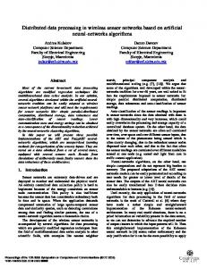
both) regarding the sensor nodes. Examples of static predicates may involve, but are not limited to, the collection of measurements from: (i) Sensors with specific identifiers; (ii) Immobile sensors in a specific area; or (iii) Sensors monitoring a specific quantity, in cases of sensor networks with diverse types of sensor nodes that monitor different quantities. Static predicates are very useful in a variety of applications and have received the focus of the bulk of past research [13, 24]. However, there is a large class of monitoring queries that cannot be expressed using static inclusion conditions. Examples include vehicle tracking and equipment monitoring applications where inclusion predicates need to be conditioned on readings taken by the sensor nodes such as noise levels or temperature readings. In its most simple form a dynamic inclusion predicate may be a condition of the form “current reading > threshold”. More complex forms may require the evaluation of a user defined function over a history of accumulated readings. We call such predicates, whose evaluation depends also on the readings taken by the nodes, as dynamic predicates as they specify which nodes should include their response in the query evaluation at each epoch (i.e., nodes whose values exceed a given threshold, or deviate significantly from previous readings). We term those monitoring queries that contain dynamic predicates as event monitoring queries (EMQs). Given a monitoring query, existing techniques seek to develop collection trees that specify the way that the data is forwarded from the sensor nodes to the Root node. Periodically these collection trees may be reorganized in order to adapt to evolving data characteristics [18]. An important characteristic of EMQs, which is not taken into account by existing algorithms that design collection trees, is that each sensor node may participate in the query evaluation, by including its reading in the query result, only a limited number of times, based on how often the inclusion conditions are satisfied. We can thus associate an epoch participation frequency Pi with each sensor node Si , which specifies the fraction of epochs that this node participated in the query result in the recent past. Given estimates of the epoch participation frequencies, one can design significantly more efficient collection trees than prior approaches. Consider the sample scenario depicted in Figure 1(a). In this figure, 36 sensor nodes are placed in a grid. The sensor identifiers appear next to each sensor node. We also distinguish the Root node at the lower left corner, a monitoring node that performs queries over the data collected by the sensor nodes. In our sample network we assume that each sensor node can communicate with its immediate horizontal, vertical or diagonal neighbors, while only node S30 can communicate with the Root node. In Figure 1(b) we depict sample estimates for the number of times each sensor node will participate in the query result within the next 100 epochs. In the above scenario, given the presented epoch participation frequencies, two interior nodes along with all the boundary nodes on the upper and right-

(a)

(b)

(c)

(d)

Figure 1: (a) Identifiers of sensors in grid arrangement; (b) Estimated number of participations in query result in 100 epochs; (c) Collection tree for MinHops algorithm. Cost = 3130 transmissions; (d) Collection tree for our algorithm. Cost = 1900 transmissions. most edges of the network always detect events, while the remaining interior nodes detect events with a lower probability, whose average value is about 5%. For the aforementioned sample scenario, in Figure 1(c) we depict a sample collection tree chosen by an algorithm, termed as MinHops that seeks to minimize the number of hops that each node’s data needs to traverse until it reaches the Root node. Next to each node we depict the actual number of transmissions that each node performed within these 100 epochs. Similarly, in Figure 1(d) we present the collection tree that our algorithms created for the evaluation of the SUM aggregate. A significant observation is that our algorithm seeks to forward the query results from nodes with high epoch participation frequencies through a limited number of interior nodes, compared to the MinHops algorithm. One can easily establish the significant reduction in the number of transmissions that our algorithm achieved (1900 vs 3130 or, equivalently, a 65% reduction).

ing sensor nodes. A good classification of aggregate functions is presented in [13], depending on the amount and type of state required in non-leaf nodes in order for them to calculate the aggregate result for the partition of descendant, in the collection tree, participating sensors. Table 2 summarizes this classification. A crucial part of the operation of our algorithms is the estimation of the amount of data that will be transmitted in a given (or candidate) collection tree. In order to accurately estimate this information, the aggregate function being used needs to be distributive, algebraic or holistic (see Table 2). Unique and content-sensitive aggregate functions can only be supported by using a worst case estimate for the amount of transmitted data. Please note that holistic aggregate queries share similar characteristics with non-aggregate queries and, thus, are treated in a similar way in our framework.

3

In this paper we seek to develop dissemination protocols for the classes of EMQs described in Section 3.1. The goal is, given the type of query at question, to design the collection tree so as to minimize either: (1) The number of transmitted messages in the network; or (2) The overall energy consumption in the network. The minimization of additional metrics of interest is discussed in Section 4.4. Our algorithms do not make any assumptions about the placement of the sensor nodes, their characteristics or their radio models.

Problem Formulation

We first introduce the types of EMQs that our framework supports and then present the optimization problems tackled in this paper. We then present the cost model used in our algorithms in order to estimate the energy consumption of a sensor node during the transmission process. 3.1 Supported Queries In Table 1 we presented the two main classes of SQL queries that our framework supports. It is important to emphasize at this point that even non-participating nodes may take part in the query evaluation process by forwarding messages towards the Root node. However, the collected values of non-participating nodes influence neither the reported query result nor its size. The first class of supported queries involve nonaggregate queries over the values of epoch participating sensor nodes. In this type of queries the amount of data transmitted by any node of the collection tree depends on the number of epoch-participating sensors that are descendants of that sensor node. The second class of supported queries involves aggregate functions over the measurements collected by the participat-

3.2

3.3

Problem Definition

Energy Consumption Cost Model

A sensor node consumes energy at all stages of its operation. However, because our algorithms do not require any significant computational effort by the sensor nodes, we ignore in the cost model used in this paper the power consumption when the sensor node is idle and the consumption due to computations. The notation that will be used in our discussion here, and later in the description of our algorithms, is presented in Table 4. Additional definitions and explanations are presented in appropriate areas of the text. We first describe the cost model used to estimate the energy consumption of a node Si during the data transmission

Category Distributive Algebraic Holistic

Type of Partial State Needed Aggregate values for descendants Aggregate values for descendants, but for different aggregate function Entire Data of descendants

Unique Content-Sensitive

Distinct Values of descendants Aggregate-Specific

State Size Constant Constant

Examples MAX, MIN, COUNT, SUM AVG

Proportional to #epoch-participating descendants Data-Dependent Data-Dependent

MEDIAN COUNT DISTINCT Histogram of Values

Table 2. Characteristics and Examples of Aggregate Function Types. Symbol Root Si Pi Di |aggr| Etri, j DEtri, j ACi, j CFi , DCFi , HCFi

Description The node that initiates a query and which collects the relevant data of the sensor nodes The i-th sensor node The epoch participation frequency of Si The minimum distance, in number of hops, of Si from the Root The size of the (non-)aggregate values transmitted by a node Energy spent by Si to transmit a new packet of |aggr| bits to S j Energy spent by Si to transmit additional |aggr| bits to S j (on an existing packet). Attachment cost of Si to a candidate parent S j Cost factors utilized by neighboring nodes of Si when estimating their attachment cost to Si

Table 4. Symbols Used in our Algorithm of |aggr| > 0 bits of data to node S j , which lies in distance disti, j from Si . The energy cost can be estimated using a linear model [17] as: Etri, j = SCi + (H + |aggr|) × (ET Xi + ERFi × disti,2 j ), where: (i) SCi denotes the energy startup cost for the data transmission of Si . This cost depends on the radio used by the sensor node; (ii) H denotes the size of the packet’s header; (iii) ET Xi denotes the per bit power dissipation of the transmitter electronics; and (iv) ERFi denotes the per bit and squared distance power delivered by the power amplifier. This power depends on the maximum desired communication range and, thus, from the distance of the nodes with which Si desires to communicate. Thus, the additional energy consumption required to augment an existing packet from Si to S j with additional |aggr| bits can be calculated as: DEtri, j = |aggr| × (ET Xi + ERFi × disti,2 j ). For the case when each sensor node receives data, we need to keep in mind that each sensor must open its radio in order to receive data or queries transmitted by neighboring nodes. This startup cost is incurred when the node wakes up from its sleep mode and, in contrast to the data transmission case, is not directly related to the reception of data (since the sensor may receive no data). Thus, this mandatory cost is not taken into account in our model. When a sensor node Si receives H + b j bits from node S j , then the energy consumed by Si is given by: Ereci = ERXi × (H + b j ), where the value of ERXi depends on the radio model. Some typical values [17] of SC, ET X , ERX and ERF are presented in Table 3.

4

Algorithm Overview

We now present our algorithms for creating and maintaining a collection tree that minimizes the desired metric

Symbol SC ET X ERF ERX

Typical Value 1µJ 50nJ/bit 100pJ/bit/m2 50nJ/bit

Table 3: Typical Radio Parameters.

(number of messages or energy consumption). We also provide detailed pseudocode in addition to a formal analysis. 4.1

Construction/Update of the Collection Tree

The algorithm is initiated with the query propagation phase. The query is propagated from the base station through the network using a flooding algorithm. In densely populated sensor networks, a node Si may receive the announcement of the query from several of its neighbors. As in [13, 24] the node will select one of these nodes as its parent node. The chosen parent will be the one that exhibits the lowest attachment cost, meaning the lowest expected increase in the objective minimization function. For example, if our objective is to minimize the total number of transmitted messages, then the selection will be the node that is expected to result in the lowest increase in the number of transmitted messages in the entire path from that sensor until the Root node (and similarly for the rest of the minimization metrics). At this point we simply note that in order for other nodes to compute their attachment cost, node Si transmits a small set of statistics Statsi and defer their exact definition for Section 4.2. The result of this process is a collection tree towards the base station that initiated the flooding process. A key point in our framework is that the preliminary selection of a parent node may be revised in a second step where each node evaluates the cost of using one of its sibling nodes as an alternative parent. Due to the nature of the query propagation, and given simple synchronization protocols, such as those specified in [13], the nodes lying k hops from the Root node will receive the query announcement before the nodes that lie one hop further from the Root node. Let RecSk denote the set of nodes that receive the query announcement for the first time during the k-th step of the query propagation phase. At step k of the query propagation phase, after the preliminary parent selection has been performed, each node Si in set RecSk , needs to consider whether it is preferable to alter its current selection and choose as its parent a sibling node within set RecSk − Si . Each node calculates a new set of statistics Statsi , based on its preliminary parent selection, and transmits an invitation, which also includes the node’s newly calculated Statsi values, that other nodes in RecSk (and only these nodes) may accept. Of course, we need to be careful at this point and make sure that at least one node within RecSk will not accept any invitation, as this would create a disconnected network and prevent nodes

from RecSk to forward their results to nodes belonging in RecSk−1 . We will achieve this by imposing a simple set of rules regarding when an invitation may be accepted by a sensor node. Let CandPari denote the set of nodes in RecSk that transmitted an invitation that Si received. Let Sm be the preliminary parent node of Si , as decided during query propagation. Amongst the nodes in CandPari , node Si considers the node S p such as the attachment cost ACi,p is minimized. If ties occur, then these are broken using the node identifiers (i.e., prefer the node with the highest id). Then S p is selected as the parent of Si instead of the preliminary choice Sm only if all of the following conditions apply: • ACi,p < ACi,m . This conditions ensures that S p seems as a better candidate parent than the current selection Sm . • ACi,p ≤ AC p,i . This conditions ensures that it is better to select S p as the parent of Si , than to select Si as the parent of S p . • If ACi,p = AC p,i , then the identifier of S p is also larger than the identifier of Si . This condition is useful in order to allow nodes to forward messages through neighbor nodes in RecSk and also helps break ties amongst nodes and to prevent the creation of loops. The collection tree may periodically get updated, either because of a significant change in data distribution or because of the addition/termination of queries in a multi-query setup discussed in section 5. Such updates are triggered by the base station using the same protocol used in the initial creation. In this case, the nodes compute and transmit their computed statistics in the same manner, but do not need to propagate the query itself. 4.2

Calculating the Attachment Cost

Determining the candidate parent with the lowest attachment cost is not an easy decision, as it depends on several parameters. For example, it is hard to quantify the resulting transmission probability of S j , if a node Si decides to select S j as its parent node. In general, the transmission frequency of S j (please note that this is different than the epoch participation frequency of the node) may end up being as high as min{Pi + Pj , 1} (when nodes transmit on different epochs) and as low as Pj (when transmissions happen on the same epochs and Pi ≤ Pj ). A commonly used technique that we have adopted in our work is to consider that the epoch participation by each node is determined by independent events. Using this independence assumption, node S j will end up transmitting with a probability Pi + Pj − Pi Pj , an increase of Pi (1 − Pj ) over Pj . Similarly, if S j−1 is the parent of S j , this increase will also result in an increase in the transmission frequency of S j−1 by Pi (1 − Pj )(1 − Pj−1 ), etc. In our following discussion, for ease of presentation, when considering the attachment cost of Si to a node S j , we will assume that the nodes in the path from S j to the Root node are the nodes S j−1 , S j−2 , . . . , S1 .

4.2.1 Minimizing the Number of Transmissions The attachment cost of Si when selecting S j as its parent node can be calculated by the increase in the transmission frequency of each link from Si to the Root node as: ACi, j = Pi + Pi (1 − Pj ) + Pi (1 − Pj )(1 − Pj−1 ) + . . . A significant problem concerning the above estimation of ACi, j is that its value depends on the epoch participation frequencies of all the nodes in the path of S j to the Root node. Since the number of these values depends on the actual distance, in number of hops, of S j to the Root node, such a solution does not scale in large sensor networks. Fortunately, there exists an alternative formula to calculate the above attachment cost. Our technique is based on a recursive calculation based on a single cost factor CFi at each node Si . In our example discussed above, the values of CFi and ACi, j can be easily calculated as: CFi ACi, j

= (1 − Pi ) × (1 +CFj ) = Pi × (1 +CFj )

One can verify that expanding the above recursive formula and setting as the boundary condition that the CF value of the Root node is zero gives the desired result. Thus, only the cost factor, which is a single statistic, is needed at each node S j in order for all the other nodes to be able to estimate their attachment cost to S j . We also need to note that the formulas presented above also address the case of non-aggregate or holistic aggregate queries. In these cases the size of the transmitted data increases proportionally to the number of each node’s epochparticipating descendants in the collection tree, as we approach the Root node. Thus, sometimes the transmitted data by a node may be split into multiple messages due to the maximum packet size. However, we first note that such cases typically occur in higher levels of the collection tree (and, thus, by a potentially small subset of the sensor nodes) and that, more importantly, our techniques seek to compute and utilize simple statistics. Our study of alternative cost models that incorporated this factor yielded only minor improvements while significantly increasing the communication cost during the collection tree formation. We thus omit such extensions from our presentation. 4.2.2 Minimizing Total Energy Consumption, Distributive and Algebraic Aggregates This case is very similar to the case described above. When considering the attachment cost of Si to a candidate parent S j , we note that additional energy is consumed by nodes in the path of S j to the Root node only if a new transmission takes place. This is because each node aggregates the partial results transmitted by its children nodes and transmits a new single partial aggregate for its sub-tree [13]. Thus, the size of the transmitted data is independent of the number of nodes in the subtree, only the frequency of transmission may get affected. Let Etri, j denote the energy consumption

when Si transmits a message to S j consisting of a header and the desired aggregate value(s) - based on whether this is a distributive or an algebraic aggregate function. The energy consumption follows the cost model presented in Section 3.3, where the PRFi value may depend on the distance between Si and S j (thus, the two indices used above). Using the above notation, and similarly to the previous discussion, the attachment cost ACi, j is calculated as: ACi, j

= Pi × Etri, j + Pi × (1 − Pj ) × Etr j, j−1 + Pi × (1 − Pj ) × (1 − Pj−1 ) × Etr j−1, j−2 + . . . = Pi × (Etri, j +CFj ),

CFi

where

= (1 − Pi ) × (Etri, j +CFj )

If one wishes to take the receiving cost of messages into account, all that is required is to replace in the above formulas the symbols of the form Etrk,p with (Etrk,p + Erec p ), since each message transmitted by Sk to S p will consume energy during its reception by S p . 4.2.3 Minimizing Total Energy Consumption, Holistic Aggregate and Non-Aggregate Queries When considering the attachment cost of Si to a candidate parent S j , we need not only consider the new messages generated in the path from S j to the Root node, but also the energy consumption due to the increase in the length of messages that would have been transmitted anyway. Please recall that the energy consumption for each transmission of |aggr| bits by Si to S j is given by: DEtri, j = |aggr| × (PT Xi + PRFi × disti,2 j ). Calculating the aforementioned number of messages is simple, as we have already discovered a similar recursive formula that estimates the attachment cost when only considering the transmission of new messages. So, we will utilize two new recursively computed statistics. The DCF value of a node will be similar to the CF value, but will use the DEtr∗,∗ transmission costs, instead of the Etr∗,∗ transmission costs used in the CF formula. The HCF value of a node will be equal to the sum of the DEtr∗,∗ values in the nodes path to the Root node. One can verify that the energy consumption due to the enlargement of messages, because of the attachment of Si to S j , that would have been transmitted anyway is: Pi × (HCFj − DCFj ). The required formulas are presented below: CFi HCFi

= (1 − Pi ) × (Etri, j +CFj ) = DEtri, j + HCFj

DCFi

= (1 − Pi ) × (DEtri, j + DCFj )

ACi, j

= Pi × (Etri, j +CFj ) + Pi × (HCFj − DCFj )

4.2.4 Summary Table 5 summarizes the statistics required to be transmitted by each node during the query propagation. Please note that the invitation phase always requires one more transmitted statistic, as the nodes need to check whether it is more beneficial to be attached to another node or the reverse (see

Minimization Metric Transmissions Energy Consumption Energy Consumption

Type of Aggregate Aggregate Non-Aggregate Distributive Algebraic Holistic Non-Aggregate

Decision

Invitation

CFi

Pi ,CFi

CFi

Pi ,CFi

CFi , HCFi , DCFi

Pi ,CFi , HCFi , DCFi

Table 5. Statistics Attached to Messages the last two rules in Section 4.1) As it can be clearly seen from this table, our algorithms utilize only a limited number of statistics, which are computed using only information transmitted by neighboring sensor nodes. Due to space constraints, the proof of the following Theorem can be found in the full paper [21]. Theorem 1 For sensor networks that satisfy the connectivity requirements of Section 3 our algorithm always creates a connected routing path that avoids loops. 4.3 Algorithm Implementation In Algorithm 1 we present the complete algorithm for the decisions of a sensor node. This algorithm is invoked both at the query propagation phase and when updating the collection tree. Each node first waits to receive the decisions by nodes that lie one hop closer to the Root node (Line 2). Based on the received decisions it performs an initial parent selection using the ProcessDecisions subroutine described in Algorithm 2 (Lines 3-4). It then calculates some necessary statistics and transmits an invitation to neighboring nodes (Lines 5-6). The node then waits (Line 7) to receive invitations from neighboring nodes and makes a final decision on its parent selection using the ProcessInvitations subroutine presented in Algorithm 3 (Lines 8-9). The node then transmits its final decision (Line 10) to neighboring nodes and ignores any received decisions or invitations until the next update period when the collection tree will be reorganized (a counter denoting the reorganization period can be attached to the queries transmitted by the Root node in order to help the nodes understand the transition to a new update period). An interesting observation that we have not mentioned so far involves the nodes with zero epoch participation frequencies. For these nodes, the computed attachment costs to any neighboring node will also be zero. In such cases we select the candidate parent which produces the lowest Etri, j +CFj + HCFj − DCFj value. This decision is expected to minimize the attachment cost, if the sensor at some point starts observing events. 4.4 Extensions In the full paper [21] we describe extensions on refining the statistics utilized by the sensor nodes. Furthermore, we show that our techniques can be easily adapted to incorporate different minimization metrics, than the ones presented in Section 3.2. For example, the formulas for minimizing the number of transmitted bits can be derived using the formulas for the energy minimization for the corresponding

Algorithm 1 BuildCollectionTree() Subroutine 1: {Si is the node being examined} 2: Wait to receive decisions by neighboring nodes −→ 3: Set Dec as the received decisions by the nodes with minimum D values (ignore other decisions).

4: 5: 6: 7: 8:

−→

k = ProcessDecisions(Dec) {Returns index of selected parent} Di = 1 + Dk Transmit invitation to neighboring nodes Wait to receive invitations by neighboring nodes −→

Set Inv as the received invitations by the nodes with D values equal to Di (ignore other invitations). −→

9: m = ProcessInvitations(Inv) {Returns index of selected parent} 10: Transmit decision 11: Ignore received decisions and invitations until next reorganization. −→

Algorithm 2 ProcessDecisions(Dec) Subroutine 1: {Si is the node being examined} 2: Select Deck as the decision with the minimum attachment cost. If Pi = 0 utilize in the calculations a non-zero value at this step to prevent all nodes from having the same (zero) attachment cost.

3: Let Sk be the sender of Deck 4: Set parent(Si ) = Sk 5: Calculate statistics (cost factors) for current node based on current parent selection 6: Return k {Index of selected parent node}

type of query (i.e., distributive, non-aggregate). In these formulas one simply has to substitute the term Etri, j with the size of a packet (including the packet’s header) and to substitute the term DEtri, j with the size of each transmitted aggregate value (thus, ignoring the header size). In the case where the goal is to maximize the minimum energy amongst the sensor nodes, the attachment cost can be derived from the minimum energy, amongst the nodes in a sensor’s path to the Root node, raised to −1 (since our algorithms select the candidate parent with the minimum attachment cost).

5

−→

Algorithm 3 ProcessInvitations(Inv, k) Subroutine 1: {Si is the node being examined} 2: {Sk is the current parent node} 3: In the following discussion, all estimations of the attachment cost utilize the same ERFi value, as discussed at the end of Section 4.2.3.

4: Select Invm as the invitation with the minimum attachment cost. If Pi = 0 utilize in the calculations a non-zero value at this step to prevent all nodes from having the same (zero) attachment cost. 5: Let Sm be the sender of Invm 6: if ACi,m ≤ ACi,k then 7: Return k {No benefit in changing parent node} 8: end if 9: Calculate ACm,i using information from Invm 10: if ACi,m > ACm,i then 11: Return k {Reverse decision is better} 12: else if ACi,m == ACm,i AND i > m then 13: Return k {Base decision on identifier} 14: end if 15: Set parent(Si ) = Sm 16: Calculate statistics (cost factors) for current node based on current parent selection 17: Return m {Index of selected parent node}

queries in order based on their identifier (i.e., from 1 to M), we demonstrate in the full paper [21] that the attachment cost ACi,k j of Si to S j regarding the k-th query is calculated as follows: • Minimizing Total Number of Transmissions.

partialPRODki, j

M

and ∏ x=1 f (x) = f (k) x (1 − Pi ), and by processing the

Using the notation

=∏ x