is a timing effect δABC = −1, but no other timing effect until the effect across A ... E appears. One should also note that it is possible that several positive timing ...
Processor Pipelines and Their Properties for Static WCET Analysis Jakob Engblom and Bengt Jonsson Dept. of Information Technology Uppsala University P.O. Box 337 SE-751 05 Uppsala, Sweden www.it.uu.se
Abstract. When developing real-time systems, the worst-case execution time (WCET) is a commonly used measure for predicting and analyzing program and system timing behavior. Such estimates should preferrably be provided by static WCET analysis tools. Their analysis is made difficult by features of common processors, such as pipelines and caches. This paper examines the properties of single-issue in-order pipelines, based on a mathematical model of temporal constraints. The key problem addressed is to determine the distance (measured in number of subsequent instructions) over which an instruction can affect the timing behavior of other instructions, and when this effect must be considered in static WCET analysis. We characterize classes of pipelines for which static analysis can safely ignore effects longer than some arbitrary threshold. For other classes of pipelines, pipeline effects can propagate across arbitrary numbers of instructions, making it harder to design safe and precise analysis methods. Based on our results, we discuss how to construct safe WCET analysis methods. We also prove when it is correct to use local worst-case approximations to construct an overall WCET estimate.
1 Introduction The purpose of Worst-Case Execution Time (WCET) analysis is to provide a priori information about the worst possible execution time of a program before using the program in a system. Reliable WCET estimates are necessary when designing and verifying embedded real-time systems, especially when used in safety-critical systems like vehicles and industrial plants. WCET estimates can be used to perform scheduling and schedulability analysis, to determine whether performance goals are met for periodic tasks, to check that interrupts have sufficiently short reaction times, to find performance bottlenecks, and for many other purposes. ∗
This work is performed within the Advanced Software Technology (ASTEC, http://www.astec.uu.se/wcet) competence center, supported by the Swedish National Innovation Systems’ Administration (VINNOVA, http://www.vinnova.se) and IAR Systems (http://www.iar.com).
WCET estimates must be safe, i.e. guaranteed not to underestimate the execution time, and tight, i.e provide acceptable overestimations. The safeness of an estimate is critical when the estimate is used in the construction of a safety-critical system. The purpose of static WCET analysis is to generate safe and tight estimates by analyzing the source code and object code of the program without executing it. The introduction of hardware features like caches and pipelines in the processors used for embedded real-time systems complicates static WCET analysis (and the measuring of execution times) by increasing the variability in execution time and by requiring more complex analysis methods. A variety of concrete analysis methods for pipelines have been proposed, ranging over cycle-accurate simulators [6, 7, 22], special-purpose models using reservation tables [4, 9, 14, 21], dependence graphs [15], abstract interpretation of pipeline behavior [8, 20], and tables of instruction execution times and inter-instruction effects [2, 3]. The timing benefit (effect) of pipelines is to a large extent due to the overlapping of pairs of adjacent instructions. This has motivated techniques that use the speedup for pairs of instructions to model the effect of pipelining [2–4, 19, 21]. The WCET is then calculated by summing execution times of instructions and subtracting the speedups. For many pipelines, there are also timing effects that only occur for sequences of three or more instructions; in this case the entire sequence has to be considered in a precise and safe timing analysis that involves the first instruction. Such long timing effects (LTEs) are introduced in [7]. In this paper, we investigate general properties of pipelines relevant for static WCET analysis, in particular the issue of how far away a single instruction in a program can affect the pipeline behavior of other instructions. Sometimes, it is enough to consider pairs of adjacent instructions, while other pipelines require that instructions quite far apart are handled in the same analysis unit. To our knowledge, this is the first work that explores the theoretical limitations of pipeline analysis. Previous WCET research has been more focussed on actually building concrete and useable WCET analysis methods than exploring the limits of analyzability. The concrete contributions of this paper are the following: – We define a mathematical model of pipeline behavior, as a basis for investigating the occurrence of LTEs. – We give general conditions under which no LTEs occur. – A central theorem shows that for a class of pipelines, all LTEs are time savings. This implies that a safe (but not necessarily precise) analysis can be performed by considering only time savings for short sequences of instructions (typically pairs). – We demonstrate that in many pipeline structures, there are cases where LTEs may occur for arbitrarily long sequences, i.e., disturbances can propagate over arbitrary distances. If such LTEs may add time, then it is hard to construct a safe and precise analysis. – We prove that in-order pipelines are not subject to the kind of timing anomalies described by Lundqvist and Stenstr¨om [16]. This indicates that local worst-case assumptions for each instruction can be used to construct the overall worst case. We do not address the issues raised by out-of-order processors, so this should only be considered a first step in our understanding of processor pipelines. 2
Paper outline: Section 2 presents the model of execution times, pairwise timing effects, and long timing effects. Section 3 presents the pipeline model built on constraints. Section 4 proves and demonstrates properties of pipelines. Section 5 discusses the implications of the properties for static WCET analysis.
2 Timing Model For the discussion in this paper, we assume that a program is represented by a set of nodes, each containing one or more instructions. Nodes are connected by edges, and sequences of nodes can be formed by following the edges. For simplicity, this presentation will assume that each node contains just a single instruction (however, the same model applies where each node is a basic block). Our goal is to statically calculate the execution time for a sequence of instructions I1 . . . Im , which is denoted by T (I1 . . . Im ). We define T (I1 . . . Im ) as the time from which I1 enters the first pipeline stage in a state where the pipeline is empty (cold pipeline) until Im leaves its last pipeline stage. An important assumption is that the same sequence of instructions always yields the same execution time. This requires that the hardware is deterministic, and that effects outside the pipeline (like cache hits and misses, variable-length instructions, etc.) are fixed by extra information in the program graph. If such information is not known, several nodes might be used to represent the same code, with different information about its execution. Techniques for such transformations are described in, for example, [6, 8]. The execution time T (I) of a single instruction I is denoted tI . To capture the timing effect of pipelines, we introduce timing effects δI1 ...Im for sequences I1 . . . Im , defined as follows. tI = T (I)
(1)
δI1 ...Im = T (I1 . . . Im ) − T (I2 . . . Im ) − T (I1 . . . Im−1 ) + T (I2 . . . Im−1 )
m≥2
(2)
We can then calculate the execution time T (I1 . . . Im ) for a sequence I1 . . . Im in terms of times and timing effects: T (I1 . . . Im ) =
m �
tIj +
j=1
�
δIi ...Ik
(3)
1≤i D(p12 , pji )) + r11 . Intuitively, this means that some stage j of some successor instruction Ii is delayed due to waiting for some corresponding stage of I1 (we assume that the first stage occurs in all instructions). Note that due to data dependences and parallel pipelines, such stalls can occur between non-adjacent instructions. Theorem 1. For a single in-order pipeline, a timing effect δI1 ...Im �= 0 can occur for a sequence of instructions I1 . . . Im , m ≥ 3 only if I1 stalls the execution of some instruction in I2 . . . Im . Proof. (Sketch) Intuitively, if I1 does not disturb any of its successor instructions, the execution of I2 . . . Im will be identical to the case when they are executed starting with I2 . The theorem can be proven by a straight-forward calculation, using the definition of stalling. A full proof is given in [6, Section 5.2.5] � � Note that for pipelines that fork, an LTE over I1 . . . Im can occur if I1 uses some resource that is not used by I2 . . . Im−1 , as shown by example in Section 4.3. 4.2
Pipelines without Positive LTEs
The central result of this section is a characterization of pipeline structures that have no positive LTEs. We say that a pipeline has the crossing critical path (CCP) property if for any constraint system model of a sequence I1 . . . Im of instructions with m ≥ 3, 1 there is a critical path P1 between p11 and pn+1 m , and a critical path P2 between p2 and n+1 pm−1 such that P1 and P2 have a common point. We assume that there is a common last step n + 1 in the pipeline (thus, we do not consider forking pipelines here). We will later give classes of pipelines that have the CCP property. The importance of CCP is that it guarantees the absence of positive LTEs. Theorem 2. For a sequence of instructions I1 . . . Im , m ≥ 2, executing on a pipeline with the CCP property, δI1 ...Im ≤ 0.
8
Proof. (Sketch) Consider the sequence I1 . . . Im and its corresponding constraint system. We shall prove that δI1 ...Im ≤ 0. Introduce the following names for points in the constraint system (see Figure 7(a)): – – – –
m, corresponding to the start of instruction I1 n, corresponding to the start of I2 n� , corresponding to the end of Im−1 m� , corresponding to the end of Im
The distances between these points form the execution times involved in the δI1 ...Im calculation as follows: T (I1 . . . Im ) = D(m, m� ) T (I2 . . . Im−1 ) = D(n, n� ) T (I1 . . . Im−1 ) = D(m, n� ) T (I2 . . . Im ) = D(n� , m) δI1 ...Im = D(m, m� ) + D(n, n� ) − D(m, n� ) − D(n, m� ) To prove that δI1 ...Im ≤ 0, we must show that D(m, m� )+D(n, n� ) ≤ D(m, n� )+ D(n, m� ). Select a critical path P1 from m to m� , shown as a dashed line in Figure 7(a), and a critical path from n to n� , shown as a solid line in Figure 7(a). By the CCP property, we can choose P1 and P2 so that they cross at some point q, dividing each of the two paths into two parts. Label the path segments by a, b, c, and d as in Figure Figure 7(a). Using the fact that the distance between two points is at least as long as any path between the points, we get the following inequalities: D(m, m� ) = a + d D(n, n� ) = b + c D(m, n� ) ≥ a + c D(n, m� ) ≥ b + d We infer that D(m, m� ) + D(n, n� ) ≤ D(m, n� ) + D(n, m� ), from which we conclude � � δI1 ...Im ≤ 0. We can now proceed to characterize pipelines with the CCP property. Theorem 3. A single in-order pipeline has the CCP property if each constraint introduced by branches (Equation (6)) and data dependences (Equation (7)) either – occurs between adjacent instructions, or – is subsumed by the basic constraints from Equations (4) and (5), as explained in Section 3 Proof. (Sketch) For single in-order pipelines without any branch or data dependency, the CCP property follows from the observation that the corresponding constraint graph is planar, and hence that critical paths cannot overtake each other without intersecting at some point. When adding constraints that represent branches and data dependences, 9
tA=6 A
T(B)=3
T(C)=6
tB=3
B
dBC= 2 T(AB)=6
(a) Execution times
T(BC)=7
T(ABC)=11
dAB =+ 1 C
dAB= -3 T(A)=6
tC=6 C (b) Timing model
Fig. 8. Long timing effect in parallel pipelines
the critical issue is whether they may allow critical paths to overtake without intersecting. As illustrated in Figure 7(b), this is not the case for constraints between adjacent instructions, since such constraints will always be included in the critical path if they make it longer. � � Note that if we have data dependences across more than two instructions, the case in Figure 7(c) can occur, and the two paths can cross without sharing a node. All branch dependences are between adjacent instructions, so the critical issue for the applicability of Theorem 3 is whether data dependences appear between non-adjacent instructions. No such dependences can appear if all data dependences in a pipeline only reach from a stage j to its predecessor stage j −1. This is thanks to the fact that since the dependence goes at most two points back in the pipeline, and all dependences beyond the non-adjacent instructions will be subsumed by the regular constraints (as illustrated in Figure 4(c)). In practice, data dependences only between adjacent instructions is a common case, thanks to data forwarding paths [11] that avoid most data dependences. Examples of processors with pipelines exhibiting this nice behavior are the ARM9 [1], NEC V850 [17] (not the V850E), Hitachi SH7700 [12], and Infineon C167 [13]. 4.3
Parallel Pipelines Cause Positive LTEs
A pipeline that forks into parallel pipelines can exhibit positive long timing effects due to interference between instructions being sent into one pipeline, if some intervening instructions are sent to some other pipeline. An example is shown in Figure 8. There might be pipelines where such effects never actually materialize, but in most real-life forking pipelines, this type of positive timing effects do occur and have to be accounted for in WCET analysis. Examples of such processors are the NEC V850E [18], MIPS R4000 [10], MicroSPARC I [9], and basically any processor employing a separate floating point pipeline. 4.4
LTEs Across Unbounded Number of Instructions
It is not in general possible to provide a bound on the length of the sequences of instructions that can exhibit long timing effects. 10
A
B
C
D
E
Data dependence from A to C
(a) The instructions A
B
C
D
D
D
E
T(ABCD...DE) = 14+2n T(ABCD...D) = 12+2n T(BCD...DE) = 11+2n T(BCD...D) = 10+2n (b) Starting with instruction A B
C
D
D
D
D
E
(c) Starting with instruction B
(d) Execution times
Fig. 9. Example of an unbounded positive timing effect
The example in Figure 9 demonstrates that we can get a positive LTE after an unbounded number of instructions. There is a data dependence between instructions A and C, which causes the execution of BCD . . . E to be different depending on whether A is executed before B or not. After an arbitary number of instructions D, we get a positive timing effect when instruction E is added, since: δA...E = 14 + 2n − 12 − 2n − 11 − 2n + 10 + 2n = +1 Thus, we can have LTEs across an arbitrary number of instructions. Note that there is a timing effect δABC = −1, but no other timing effect until the effect across A . . . E appears. One should also note that it is possible that several positive timing effects occur from the same disturbance [6]. 4.5
Absence of Timing Anomalies
Using the model in Section 3, we can also establish a different but important property of in-order pipelines, the absence of timing anomalies, as introduced by Lundqvist and Stenstr¨om [16]. Given a sequence of instructions I1 . . . Im , when we change the execution time of the first instruction by adding n cycles, we will get a new execution time for the sequence. If this time is less than the previous time, or the new time is more than n cycles longer than the previous time, we have a timing anomaly. We translate this property into our model by assuming that precisely one pipeline stage for I1 is extended to take more cycles. By example, Lundqvist and Stenstr¨om demonstrated that out-of-order processors can suffer from timing anomalies. Here, we show that for pipelines that can be modeled by our constraint systems (in-order pipelines), such effects cannot occur. Note that 11
branch prediction coupled with speculative cache fetches can cause timing anomalies, regardless of the simplicity of the pipeline, as demonstrated for the Coldfire 5307 [8]. To avoid timing anomalies, we require that a processor is free from all kinds of dynamic scheduling and speculative processing. The important consequence of timing anomalies is that if anomalies occur, we cannot use the simplifying assumption that the worst-case execution time for the program can be derived by assuming worst-case execution times for each individual instruction. Otherwise, every possible pipeline and/or cache state has to be considered, which is very complex [8]. Theorem 4. For in-order pipelines, no timing anomalies can appear when we increase the execution time of an instruction. Proof. The original execution time for I1 . . . Im corresponds to the critical path in a constraint system C1 . We increase the execution time by increasing the time for I1 to complete one of its stages, obtaining a new constraint system C2 , where some r1j is bigger than in C1 . The new execution time for I1 . . . Im corresponds to some critical path in constraint system C2 . If the arrow with r1j was on the critical path before, the execution time will increase by k cycles, d = k. If it was not, and now is included, the time will increase by at most k. If it is not on the critical path of either C1 and C2 , d = 0. Thus, 0 ≤ d ≤ k, and no timing anomaly can appear. � � Theorem 5. For in-order pipelines, no timing anomalies can appear when we decrease the execution time of an instruction. Proof. Analogous to the proof of Theorem 4 [6].
� �
5 The Safety of WCET Analysis To perform safe WCET analysis for pipelines, we need to make sure that no positive LTEs are missed. If no positive LTEs can occur at all, as is the case for the processors with the CCP property, any timing model that considers instructions, pairs of instructions, etc. is safe, since there are no positive LTEs that can be missed. However, for many types of processors, positive LTEs can occur, and there are several ways of handling them. For approaches only analyzing adjacent pairs of instructions, the presence of positive LTEs makes it necessary to use conservative approximations. Such an approximate model would overestimate the execution time over shorter sequences, in order to make sure that the total execution time when LTEs are taken into account is not underestimated. One way to construct such a model is to use reservation tables and consider their pairwise concatenation, but not allow the instruction profiles to change their shape when concatenated. This means that stalls will not materialize, as each instruction will execute as it would in isolation. Thus no long effects can occur within a pipeline, according to Theorem 1. To avoid the potential of LTEs resulting from parallel pipelines, it is 12
tA=6 A dAB= -2 T(A)=6
T(AB)=7
(a) Execution times
T(B)=3 Fake pipeline stage uses inserted to make the analysis safe
T(C)=6
tB=3
B
dBC= 1 T(BC)=7
tC=6 C
Execution time for just AB is overestimated, 7 cycles rather than 6 For entire sequence ABC, execution time in the model is 12 cycles, an overestimation
(b) Timing model
Fig. 10. Pairwise conservative model for Figure 8
necessary that each instruction (or basic block) use every pipeline stage, as proposed in [19] 1 . Also, if there are data dependences between non-adjacent instructions it is necessary to account for the worst possible delay due to data waits, in each pair of instructions. Note that just concatenating instructions pairwise without stalls [4, 21] is not necessarily safe for parallel pipelines. Figure 10 shows how the case in Figure 8 would be modeled with this type of approximation: node A would not be allowed to completely overlap node B (as shown for the sequence AB), which makes the timing effect between the nodes −2 instead of −3. Thus, the positive timing effect of the interference between A and C is taken early, on the edge between A and B, which is safe but pessimistic. If a processor has instructions that can execute for quite a long time in parallel to other instructions, this type of approximation is likely to give very high overestimations. In our WCET analysis method based on examining sequences of nodes [6, 7], it is critical to define correct criteria for the termination of the search that finds all (positive) LTEs. If those criteria are wrong, we might get an underestimated WCET. In practice, this type of analysis works very well for simple processors. Another approach maintains multiple pipeline states for each basic block, and in each step tries to prune the states that cannot result in the longest execution time [14]. This pruning operator has to consider the potential of LTEs to be correct. There are some analysis approaches where the pipeline behavior is modeled along paths consisting of many basic blocks [9, 22] (usually, this means that several different paths between two points in the code are analyzed). Inside each path, LTEs are absorbed with perfect precision, but where paths are concatenated, approximations that cover all possible LTEs have to be used. A different philosophy is to maintain all possible states of the pipeline for each node in the analysis, without attempting to prune the set of pipeline states [8, 20]. In such approaches, the presence of LTEs will mean an increased analysis complexity (as each instruction will be subject to more different states). This approach is not dependent on the absence of timing anomalies and should find all LTEs. The resulting analysis is very expensive, however [8]. 1
The placement of such extra pipeline stages is qiute important to achievable precision, and has to be carefully considered for each pipeline
13
6 Conclusions In this paper, we have presented a mathematical model of instruction execution on inorder single-issue pipelined processors. We have used this model to examine the timing of instructions from the perspective of static worst-case execution time (WCET) analysis, especially considering timing effects between non-adjacent instructions (long timing effects, LTEs). There are negative LTEs, which can be safely ignored, and positive LTEs that add instruction time to a sequence of instructions, and that have to be accounted for in a safe analysis. Even simple pipelines can exhibit LTEs across arbitrary numbers of instructions, which makes it necessary for static WCET analysis to consider more than pairs of instructions. For many pipelines, all LTEs are negative, which means that they can be ignored safely, at the cost of lower precision. Measurements indicate that (we have experimented with the NEC V850E processor) ignoring all negative LTEs can give overestimations of up to 20% of the execution time of a program [6]. For processors with parallel floating point pipelines, the effect could be much greater. Another result obtained using our pipeline model is that in-order single-issue processors are not subject to timing anomalies, which indicates that it is possible to use local worst-case assumptions to derive a global worst-case execution time. This allows for efficient static analysis, since we do not have to consider all possible execution times for each instruction in order to find the WCET. The results in this paper indicates that certain processors are better suited for use in predictable systems. For example, the timing of a processor without timing anomalies and only negative LTEs is very easy to analyze compared to a processor with positive LTEs and timing anomalies. It would be interesting to try to design a high-performance high-predictability processor for embedded real-time systems. In conclusion, we reached a better understanding of how to construct safe static WCET analysis methods for pipelined processors, and have identified some non-trivial problems related to the achievable safety and precision of WCET analysis. This provides static WCET analysis with a firmer theoretical background, which will help us build better analysis methods. We hope to continue this work by extending the pipeline model to more classes of pipelines and continue the investigation into pipeline properties.
References 1. ARM Ltd. ARM 9TDMI Technical Reference Manual, 3rd edition, March 2000. Document no. DDI 0180A. 2. P. Atanassov, R. Kirner, and P. Puschner. Using Real Hardware to Create an Accurate Timing Model for Execution-Time Analysis. In Proc. IEEE Real-Time Embedded Systems Workshop, held in conjunction with RTSS 2001, December 2001. 3. I. Bate, G. Bernat, G. Murphy, and P. Puschner. Low-level Analysis of a Portable Java Byte Code WCET Analysis Framework. In Proc. 7th International Conference on Real-Time Computing Systems and Applications (RTCSA’00), pages 39–48. IEEE Computer Society Press, December 2000.
14
4. A. Colin and I. Puaut. A Modular and Retargetable Framework for Tree-Based WCET Analysis. In Proc. 13th Euromicro Conference on Real-Time Systems, (ECRTS’01). IEEE Computer Society Press, June 2001. 5. Rina Dechter, Itay Meiri, and Judea Pearl. Temporal constraint networks. Artifical Intelligence, 49:61–95, 1991. 6. J. Engblom. Processor Pipelines and Static Worst-Case Execution Time Analysis. PhD thesis, Dept. of Information Technology, Uppsala University, April 2002. Acta Universitatis Upsaliensis, Dissertations from the Faculty of Science and Technology 36, http://publications.uu.se/theses/91-554-5228-0/. 7. J. Engblom and A. Ermedahl. Pipeline Timing Analysis Using a Trace-Driven Simulator. In Proc. 6th International Conference on Real-Time Computing Systems and Applications (RTCSA’99). IEEE Computer Society Press, December 1999. 8. C. Ferdinand, R. Heckmann, M. Langenbach, F. Martin, M. Schmidt, H. Theiling, S. Thesing, and R. Wilhelm. Reliable and Precise WCET Determination for a Real-Life Processor. In Proc. First International Workshop on Embedded Software (EMSOFT 2001), LNCS 2211. Springer-Verlag, October 2001. 9. C. Healy, R. Arnold, F. Mueller, D. Whalley, and M. Harmon. Bounding pipeline and instruction cache performance. IEEE Transactions on Computers, 48(1), January 1999. 10. J. Heinrich. MIPS R4000 Microprocessor User’s Manual. MIPS Technologies Inc., 2nd edition, 1994. 11. J. L. Hennessy and D. A. Patterson. Computer Architecture A Quantitative Approach. Morgan Kaufmann Publishers Inc., 2nd edition, 1996. ISBN 1-55860-329-8. 12. Hitachi Europe Ltd. SH7700 Series Programming Manual, September 1995. 13. Infineon. Instruction Set Manual for the C166 Family, 2nd edition, March 2001. 14. S.-S. Lim, Y. H. Bae, C. T. Jang, B.-D. Rhee, S. L. Min, C. Y. Park, H. Shin, K. Park, and C. S. Ki. An Accurate Worst-Case Timing Analysis for RISC Processors. IEEE Transactions on Software Engineering, 21(7):593–604, July 1995. 15. S.-S. Lim, J. H. Han, J. Kim, and S. L. Min. A Worst Case Timing Analysis Technique for Multiple-Issue Machines. In Proc. 19th IEEE Real-Time Systems Symposium (RTSS’98), December 1998. 16. T. Lundqvist and P. Stenstr¨om. Timing Anomalies in Dynamically Scheduled Microprocessors. In Proc. 20th IEEE Real-Time Systems Symposium (RTSS’99), December 1999. 17. NEC Corporation. V850 Family 32/16-bit Single Chip Microcontroller User’s Manual: Architecture, 4th edition, 1995. Document no. U10243EJ4V0UM00. 18. NEC Corporation. V850E/MS1 32/16-bit Single Chip Microcontroller: Architecture, 3rd edition, January 1999. Document no. U12197EJ3V0UM00. 19. G. Ottosson and M. Sj¨odin. Worst-Case Execution Time Analysis for Modern Hardware Architectures. In Proc. ACM SIGPLAN Workshop on Languages, Compilers and Tools for Real-Time Systems (LCT-RTS’97), June 1997. 20. J¨orn Schneider and Christian Ferdinand. Pipeline Behaviour Prediction for Superscalar Processors by Abstract Interpretation. In Proc. ACM SIGPLAN Workshop on Languages, Compilers and Tools for Embedded Systems (LCTES’99), May 1999. 21. Friedhelm Stappert. Predicting pipelining and caching behaviour of hard real-time programs. In Proc. of the 9th Euromicro Workshop on Real-Time Systems. IEEE Computer Society Press, June 1997. 22. D. Ziegenbein, F. Wolf, K. Richter, M. Jersak, and R. Ernst. Interval-Based Analysis of Software Processes. In Proc. ACM SIGPLAN Workshop on Languages, Compilers and Tools for Embedded Systems (LCTES’2001), June 2001.
15