Turku Centre for Computer Science ... statements on disjoint state spaces, where program statements are modeled .... The convention of using primed variables ...
Programs on Product Spaces Ralph-Johan Back
� Abo Akademi University, Department of Computer Science Lemminkaisenkatu 14 A, FIN-20520 Turku, Finland email: backrj@abo.
Joakim von Wright
� Abo Akademi University, Department of Computer Science Lemminkaisenkatu 14 A, FIN-20520 Turku, Finland email: jwright@abo.
Turku Centre for Computer Science TUCS Technical Report No 143 November 1997 ISBN 952-12-0096-0 ISSN 1239-1891
Abstract We study program states that are described as tuples, i.e., product state spaces. We show how to add program variables and assignment notation to simply typed lambda calculus in order to describe functions, relations and predicate transformers on such spaces in a concise way. We de ne an operator on program statements that describes the independent execution of statements on disjoint state spaces, where program statements are modeled as predicate transformers. We study the algebraic properties of this product operator, in particular the basic monotonicity and distributivity properties that the operator has. We also consider how to extend the state space by adding new state components, and show how this is modeled using the product operator.
TUCS Research Group
Programming Methodology Research Group
1 Introduction In imperative programming, a program state typically consists of a number of components (program variables, modules, etc.) that can be updated and accessed independently of each other. This allows us to use incremental updates, like assignment statements, to change only part of the state. A natural model for a state with components is a tuple of values. In this paper, we consider how programs on such state spaces can be described. In particular, this view of program states allows us to de ne a general product operator on programs, which models the independent execution of programs on disjoint sets of state components. For example, a multiple assignment of the form x; y := x+1; y ?1 can be seen as updating the two program variables x and y in parallel (independently, simultaneously). A simple assignment like x := x +1 can be seen as executing a skip statement on all the other program variables, in parallel with the updating of x. This notion of parallelism makes it possible to analyse the statement independent of the context of program variables that it occurs in. Programs can be modeled in di�erent ways. We consider three basic models, state transformers or total functions on the state space, state relations or relations between state spaces, and predicate transformers or functions from postconditions on the state space to preconditions on the state space. All these models have been proposed for describing the mathematical meaning of programs, and are of increasing strength. Total functions are really too restrictive, because we cannot even model nontermination of program statements. Relations provide a more expressive framework, where either nondeterminism or nontermination (but not both) can be modeled. Predicate transformers provide the most expressive model, allowing us to model two di�erent kinds of nondeterminism, angelic and demonic, as well as distinguishing between aborting and miraculous termination, where aborting termination can be used to model nontermination. We express these models for programs within the general framework of re nement calculus. We de ne product operators for state transformers, state relations, and predicate transformers, and investigate the properties of these operators. We concentrate on the properties of the product operator on predicate transformers, showing that it has many properties that are useful in re nement. Examples of such properties are monotonicity and certain homomorphism properties, distributivity with respect to other program constructs and preservation of data re nement. The product is also used to de ne an operation that extends a statement into a larger context by adding new state components. We also describe how the product operator works in a more syntactic 1
context. We propose a simple syntactic extension to typed lambda calculus, by introducing the notions of program variables, assignment statements and variable declarations for functions and relations on product spaces. This allows us to describe state transformers and state relations in a concise way. The idea of de ning a parallel operator in a predicate transformer framework is old, and many syntactically oriented solutions have been proposed. However, attempts to generalise the parallel assignment x := e k y := e0 to a general parallel operator generally give rise to complicated de nitions [1]. Product operators on predicate transformers have been investigated previously by other researchers. Martin [8] and Naumann [9] take a category-theoretic approach, de ning (among other things) the same product operator as we investigate here. However, their investigation are purely algebraic, while we concentrate more on the role of the product in the context of re nement and we also focus on syntactic aspects of programs on product spaces. Back and Butler [2] also investigate various product and sum constructs for predicate transformers. However, the product operator that we concentrate on here is not in the centre of their focus. The rest of the paper is organised as follows. In Section 2 we consider functions and relations on product spaces. We introduce an assignment notation that allows functions and relations to be expressed in a simple way. In Section 3 we describe how program statements are modeled as predicate transformers and we extend the assignment notation to predicate transformers. In Section 4 product operators are described and their basic properties are investigated. This section adds some new results to those already obtained by other researchers. In Section 5 we derive distributivity properties of the product operator on statements and apply it to data re nement. Extension is described in Section 6 and its independence of the product is investigated in Section 7. Finally, Section 8 contains conclusions and some discussion.
2 Functions and relations on product spaces Let us start by looking at state predicates, state transformers and state relations, when the state space � is a product space, � = �1 � : : : � �n . We use the notation of simply typed classical higher order logic. In particular, we use (tupled) lambda notation for functions, so, e.g., (�x; y � x + y) is a function which takes a pair of arguments and returns their sum. Function application is written as an in x dot (as f: x). We use Bool to stand for the set of truth values F and T, and � for boolean equivalence. In proofs, we use a calculational format. Only the most important proofs are shown in the paper; the other proofs can be found in the Appendix. 2
A state transformer is a function f : � ! � that maps states to states. We write (forward) composition of state transformers as f ; g (so (f ; g): � = g: (f: �)), and write id for the identity state transformer (so id: � = �). A state predicate is a function p : � ! Bool. Since a predicate corresponds to a set of states, we also use set notation for predicates. Thus, � 2 p can be expressed as p: � = T, and we write \ for conjunction, [ for disjunction and � for the inclusion (strength) ordering. The empty (everywhere false) predicate is false and the full (everywhere true) predicate is true. Note that these constants are all de ned by pointwise extension of the corresponding boolean constants, e.g., p \ q = (�� � p: � ^ q: �) and p � q � (8� � p: � ) q: �). A state relation is a function R : � ! � ! Bool. A relation thus maps a state to a predicate. We say that R relates � to �0 if �0 2 R: �, i.e., if R: �: �0 � T. We use the set operators for relations also, de ned by pointwise extension from predicates. Thus, for example, Q [ R = (�� �0 � Q: �: �0 _ R: �: �0). The empty relation is False and the full relation is True. Relational composition is de ned in the usual way: (P ; Q): �: �0 holds if and only if (9 � P: �: ^ Q: : �0).
2.1 Assignment notation
State spaces of the form � = �1 � : : : � �n can be quite di�cult to handle when n is large. The usual lambda notation is not particularly well suited for describing functions and relations on such state spaces. For instance, a typical function might be (�a; b; c; d; e; f; g; h � a; b; c; a + b; e; f; g; h) with most of the state components unchanged. The lambda notation forces us to list all components of the nal state, whether these have been changed or not. The assignment notation that is used in programming languages is much better here. The change above could be described simply as
d := a + b provided the context makes it clear that the state components are named a; b; c; d; e; f; g; h. The implicit understanding is that only component d is changed, while the other state components remain unchanged. We introduce an assignment notation of this kind as a syntactic sugaring for ordinary lambda terms, in the following way. Consider the function f : �1 � : : : � �n ! �1 � : : : � �n , where f = (�u1; : : :; un � t1; : : :; tn) 3
The function f replaces the old components u1; : : :; un by new components t1; : : : ; tn of the same type. We want to indicate that certain components are changed and given new values, while all other components remain unchanged. We introduce the (functional) assignment notation for this: (�u � x1; : : :; xm := t1; : : :; tm) =^ (�u � u[x1; : : : ; xm := t1; : : :; tm]) where u = u1; : : :; un. An example is (�a; b; c � a; c := a + b; a ? c) = (�a; b; c � a + b; b; a ? c) Here a and c (the rst and third state components) are given new values, while b (the second state component) is unchanged. Note that the assignment notation is just syntactic sugaring; we can always rewrite an assignment as an ordinary lambda term. A relation R : �1 � : : : � �m ! �1 � : : : � �m ! Bool can be written in lambda notation as (�x1; : : : ; xm � �y1; : : : ; ym � b) for some boolean term b. Using set notation we can also write this as (�x1; : : :; xm � fy1; : : :; ym j bg) where b can contain free occurrences of the variables in the lists x = x1; : : :; xm and y = y1; : : : ; ym (as well as other free variables). We extend the assignment notation to relations, as follows: (�u � x := y j b) =^ (�u � fu[x := y] j bg) An example is (�a; b; c � a; c := a0; c0 j a + b = a0 ? c0) = (�a; b; c � fa0; b; c0 j a + b = a0 ? c0g) The fact that b is not changed in the relation is shown by having the same b in the bound variable position in the set. The convention of using primed variables for components of the nal state makes assignments easy to read.
2.2 Program variables
The assignment notation does not solve the whole problem with verbose descriptions of statements. A typical statement term is, e.g., (�x; y; z � x := x + y) ; (�x; y; z � z := 0) ; (�x; y; z � y := z ? x) 4
Each function term here is a lambda abstraction. In this case we have used the same bound variable names in each abstraction. However, nothing prevents us from renaming these bound variables, using �-conversion. For instance, the following function term is equal to the previous one: (�y; z; x � y := y + z) ; (�x; z; y � y := 0) ; (�z; x; y � x := y ? z) This freedom of renaming bound variables that denote state components is obviously not desirable, since it makes it more di�cult to understand the intended e�ect of the predicate transformer. A consistent naming of the state components is clearly preferable. Because the same bound variables are used in all components, we can move the lambda abstraction to the outermost level of the construct. Let us write (var x; y; z � (y := y + z) ; (z := 0) ; (x := y ? z)) to express that each function term is to be understood as a lambda abstraction over the bound variables x; y; z. We understand this as a shorthand for the term where the var x; y; z construct has been distributed inside to each basic function term, creating a lambda abstraction over these same variables: (var x; y; z � (y := y + z) ; (z := 0) ; (x := y ? z)) = (�x; y; z � y := y + z) ; (�x; y; z � z := 0) ; (�x; y; z � x := y ? z) The notation (var u � t) thus enforces a consistent naming of state components in a state transformer term. Let us look at this abbreviation in somewhat more detail. We consider rst state predicates. Let b be boolean term. We de ne (var u � b) =^ (�u � b) Thus program variable declaration var u is here just a shorthand for lambda abstraction. The way in which predicates are de ned as pointwise extensions of truth values then implies that var u distributes inside a boolean term: (var u � T) = true (var u � F) = false (var u � b ^ b0) = (var u � b) \ (var u � b0) (var u � b _ b0) = (var u � b) [ (var u � b0) ::: = ::: As an example, we have that (var x; y � (x � z) ^ T) = (�x; y � x � z) \ true 5
Note that the predicate de ned here has a free variable z. We can use this notation also for quanti ed expressions, where we have that (var u � (8x � b)) = (\x � (var u � b)) (var u � (9x � b)) = ([x � (var u � b)) We assume here that x does not occur in the list of variables u.
2.3 Function statements
Now let us introduce a small language of function statements for state transformers: a ::= x := t j a1 ; a2 Here x = x1; : : :; xm is a list of distinct variables and t = t1; : : :; tm is a corresponding list of terms, m � 0, such that xi and ti are of the same type, for i = 1; : : : ; m. We de ne the program variable notation for this language, as follows: (var u � x := t) =^ (�u � x := t) (var u � a1 ; a2) =^ (var u � a1) ; (var u � a2) We assume that the variables in x are all included in u. Thus, the program variable declaration also distributes over forward functional composition. Assignment to an empty list of variables is permitted as a special case. We have that (var u � � := �) = id, where � stands for the empty list.
2.4 Relation statements
In the same way, we can use the program variable notation for relations. We de ne rst a small language for relation statements: r ::= (x := x0jt) j :r1 j r1 ^ r2 j r1 _ r2 j r1 ; r2 : : : We then de ne the program variable notation in a similar way as above, so that the program variable declaration distributes over the relation operators: (var u � x := x0 j b) =^ (�u � x := x0 j b) (var u � :r) =^ :(var u � r) (var u � r ^ q) =^ (var u � r) \ (var u � q) (var u � r _ q) =^ (var u � r) [ (var u � q) (var u � r ; q) =^ (var u � r) ; (var u � q) ::: ::: 6
Again, we assume that the variables in x are included in in u. There are three special cases for relations, which we can compute from the above de nitions: (var u � u := u0 j T) = True (var u � u := u0 j F) = False (var u � � := � j t) = j(var u � t)j Here jpj stands for the relation (�� �0 � � = �0 ^ p: �), where p is a predicate.
3 Predicate transformers as program statements We assume that the reader is familiar with the weakest precondition semantics of simple imperative programming languages [6] and with the basic notions of program re nement [3, 4]. We here quickly describe the notions of states, predicates and predicate transformers used in this paper, and how they are formalised.
3.1 Predicate transformers
A predicate transformer is a function that maps predicates to predicates. We use Ptran(�; ?) for the set of functions that map predicates in ? ! Bool to predicates in � ! Bool. Here � is the initial state space and ? the nal state space. We take predicate transformers to model programs according to a weakest precondition intuition; if S is a predicate transformer and q a predicate over its nal state space (a postcondition) then the predicate S: q describes those initial states from which execution of S is guaranteed to terminate in a state in q. If � 2 S: q, then we say that S establishes postcondition q in initial state �. The predicate transformers (for given state spaces) form a complete boolean lattice. Basic operators are de ned by pointwise extension from predicates. For example, S v S 0 = (8q � S: q � S 0: q) and S uS 0 � (�q � S: q \S 0: q). The bottom element is abort = (�q � false) and the top element is magic = (�q � true). Since predicate transformers are functions, we also have a composition operator, (S ; S 0): q = S: (S 0: q), and a unit, skip. Thus, the booleans, state transformers, predicates, relations and predicate transformers form a hierarchy with uniform structure and notation; the so called predicate transformer hierarchy [5]. 7
The meet operator in Ptran(�; ?) can be interpreted as a demonic choice operator; S u S 0 establishes q if and only if both S and S 0 establish q. Dually, the join operator models angelic choice; S t S 0 establishes q if and only if at least one of S and S 0 establishes q. The bottom element abort establishes no postcondition, not even true. Dually, the top element magic establishes all postconditions, even false. This is often referred to as miraculous termination. We classify predicate transformers according to basic homomorphism properties. A predicate transformer S is conjunctive if it distributes over nonempty conjunctions, i.e., if S: (\ i 2 I � qi) = (\ i 2 I � S: qi) for arbitrary nonempty collections fqi j i 2 I g of predicates. Intuitively speaking, a predicate transformer is conjunctive if it models a program statement with only demonic nondeterminism. Dually, S is disjunctive (angelically nondeterministic) if S: ([ i 2 I � qi) = ([ i 2 I � S: qi). Furthermore, S is strict if S: false = false and terminating if S: true = true. Finally, we say that S is universally conjunctive if it is conjunctive and terminating and S is universally disjunctive if it is disjunctive and strict.
3.2 Basic predicate transformer constructs
Meet, join and composition (which is interpreted as sequential composition) give us means of combining predicate transformers. However, we also need a notation for basic statements to be used as building blocks for constructing more complicated statements. We de ne the following basic predicate transformers, where p is a state predicate, f a state transformer and R a state relation: [p]: q = :p [ q fpg: q = p \ q hf i: q = (�� � q: (f: �)) [R]: q = (�� � R: � � q) fRg: q = (�� � R: � \ q =6 ;)
(guard ) (assert ) (functional update ) (demonic update ) (angelic update )
Intuitively, the guard statement [p] and the assert statement fpg both test whether the condition p holds in the present state. If the condition holds, then both act as a skip, i.e., do not change the state. If the condition does not hold, then the guard statement terminates miraculously while the assert statement aborts. The functional update statement applies the function f to the present state to get the new state. The demonic update [R] and the angelic update fRg both give as a new state some state that is related by R to the present state. The choice of the new state is in the rst case assumed 8
to be done demonically, in the second case angelically. If there is no state that can be reached by R from the present state, then the demonic update terminates miraculously, while the angelic update aborts. For a more detailed intuitive justi cation of these constructs, we refer to Back and von Wright [5]. In addition to an appealing intuition, they also have simple homomorphism properties. These include monotonicity properties as well as lattice homomorphism and functor properties. The following are a few examples:
P � Q ) [P ] v [Q] [P ] u [Q] = [P [ Q]
p � q ) fpg v fqg fP g ; fQg = fP ; Qg
For a full treatment of algebraic properties of the basic predicate transformers we also refer to [5].
3.3 Normal forms
The basic notation provides normal forms for di�erent classes of predicate transformers
Lemma 1 Assume that S is a predicate transformer. (a) If S is monotonic then it can be written in the form fP g ; [Q] for some relations P and Q. (b) If S is conjunctive then it can be written in the form fpg ; [Q] for some predicate p and some relation Q. (c) If S is universally conjunctive then it can be written in the form [Q] for some relation Q. This normal form theorem is proved in [10]. Dual results to (b) and (c) also hold for disjunctive and universally disjunctive predicate transformers. These normal forms allow us to model programs that do not fall into the simple basic categories that we have chosen (total functions, relations or predicate transformers). For instance, conjunctive predicate transformers are often used to model programs with possible nontermination and (demonic) nondeterminism. Partial functions can be seen as a subclass of relations (functional relations), whereas relations again can be embedded as a subclass of predicate transformers (the universally conjunctive predicate transformers). 9
3.4 Statements The program variable notation is used also for describing predicate transformers, by postulating that var u also distributes over the predicate transformer constructors described above. Let us rst de ne a small language of statements:
s ::= fbg j [b] j hai j frg j [r] j s1 ; s2 j s1 u s2 j s1 t s2 j : : : Here we assume that b is a boolean term, a is a function statement, r is a relation statement and s1 and s2 are statements. We then de ne the program variable declaration in the same way as above: (var u � [b]) =^ [(var u � b)] ::: ::: ^ � (var u frg) = f(var u � r)g (var u � s1 ; s2) =^ (var u � s1) ; (var u � s2) ::: ::: The three special cases that we get are as follows: (var u � fFg) = abort (var u � h� := �i) = skip (var u � fTg) = magic A simple example of a statement is (var u � fx � 0g ; (hx := x + yi t hx := x + 1i) Applying the rules above, this describes the predicate transformer
f�u � x � 0g ; (h�u � x := x + yi t h�u � x := x + 1i) (from now on, we drop parentheses nested inside other brackets). The advantage of this notation becomes quite clear in larger statements, where there are many state components and many subterms. It gives us the traditional program variable and assignment notation as a simple syntactic sugaring over standard lambda terms in higher order logic. 10
4 Product operators The fact that we are working on a state space that is a tuple means that it is feasible to consider manipulating two disjoint parts of the state space in parallel, independently of each other. We now show how to de ne independent operations on the state for the basic mathematical entities that we have introduced to model programs: predicates, relations, state transformers and predicate transformers. Let p1 : �1 ! Bool and p2 : �2 ! Bool be two predicates. Their product p1 � p2 : �1 � �2 ! Bool is de ned by (p1 � p2): (�1; �2) =^ p1 : �1 ^ p2: �2 Thus, products correspond to componentwise testing for truth. Note that p1 � false = false � p2 = false and true � true = true. For relations P1 : �1 ! ?1 ! Bool and P2 : �2 ! ?2 ! Bool, we similarly de ne the product P1 � P2 : �1 � �2 ! ?1 � ?2 ! Bool as follows: (P1 � P2): (�1; �2): ( 1; 2) =^ P1: �1: 1 ^ P2: �2: 2 Thus the product of two relations is the pointwise extension of the product of two predicates: (P1 � P2): (�1; �2): = P1: �1 � P2: �2 Furthermore, True � True = True and Id � Id = Id. For the bottom element we have the stronger P1 � False = False � P2 = False. In fact, the following result holds, which shows that we cannot in general recover predicates from products by projection: Lemma 2 Let p and q be two predicates. Then p � q = false � p = false _ q = false The proof of Lemma 2 is straightforward, but we include it as an example of the proof format we use. Proof
p � q = false � fde nition of product and falseg (8� �0 � :(p: � ^ q: �0)) ) fde Morgan and quanti er rulesg (8� � :p: �) _ (8�0 � :q: �0) � fde nition of falseg p = false _ q = false 11
2
For state transformers f1 : �1 ! ?1 and f2 : �2 ! ?2 the product f1 � f2 : �1 � �2 ! ?1 � ?2 is de ned by (f1 � f2): (�1; �2) =^ (f1: �1; f2: �2) Note that id � id = id. The product of two state functions is thus a state function on the combined state space, where each function is applied on its state component independently of the other component. The algebraic properties of the product operators on predicates, functions and relations are standard and easily derived, so we will not study them any further here. Instead we concentrate on the product of predicate transformers and its algebraic properties.
4.1 Predicate transformer product
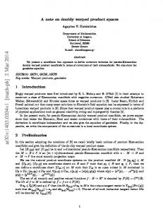
The product of two predicate transformers S1 : Ptran(�1; ?1) and S2 : Ptran(�2; ?2) is written S1 � S2 : Ptran(�1 � �2; ?1 � ?2 ). It is de ned as follows, for q : ?1 � ?2 ! Bool and �1 : �1 and �2 : �2: (S1 � S2): q: (�1; �2) =^ (9q1 q2 � q1 � q2 � q ^ S1: q1: �1 ^ S2: q2: �2) Intuitively, this means that S1 � S2 establishes the postcondition q � ?1 � ?2 in initial state (�1; �2), if there is a "rectangular" subset q1 � q2 of q such that S1 establishes q1 in �1 and S2 establishes q2 in �2 independently. The product operator for predicate transformers is illustrated in Figure 1. To avoid excessive parentheses, we give the product operator lower precedence than sequential composition. Thus we can write (S1 ; S2) � (S3 ; S4) as S1 ; S2 � S3 ; S4. We note that product preserves monotonicity, as well as all four basic homomorphism properties:
Theorem 3 Let S1 : Ptran(�1; ?1) and S2 : Ptran(�2; ?2) be two predicate transformers. Then S1 � S2 preserves monotonicity, strictness, termination, conjunctivity and disjunctivity.
Proof This result is proved (in an indirect way) by Back and Butler [2], We
include a direct proof in the Appendix. 2 Products of strict monotonic predicate transformers also preserve products, in the following sense. 12
Γ2 q
q2
( σ1 ,σ2 )
q1
Γ1
Figure 1: Product of predicate transformers
Theorem 4 Let S1 and S2 be two strict monotonic predicate transformers. Then
(S1 � S2): (p � q) = S1: p � S2: q for arbitrary predicates p and q.
Proof First assume S1 : p0 : �1 ^ S2 : q 0: �2 ^ p0 � q 0 � p � q . Then
p0: � ) fS2: q0: �2 implies q0 6= false, by strictnessg (9�0 � p0: � ^ q0: �0) ) fp0 � q0 � p � q, de nitiong (9�0 � p: � ^ q: �0) ) fpredicate calculusg p: � which (with a similar argument for q and q0) shows that S1: p: �1 ^ S2: p: �2 ^ p0 � q0 � p � q ) p0 � p ^ q0 � q (* ) Now, (S1 � S2): (p � q): (�1; �2) 13
� fde nitions of productsg (9p0 q0 � p0 � q0 � p � q ^ S1: p0: �1 ^ S2: q0: �2) � f( by choosing p0 := p, q0 := q and ) by (*), monotonicityg S1: p: �1 ^ S2: q: �2 � fde nitiong (S1: p � S2: q): (�1; �2)
and the proof is nished. 2 The following counterexample shows that strictness is in fact required in Theorem 4. We have (magic � skip): (false � false) = true because magic � skip = magic (see Theorem 9 below), but magic: false � skip: false = false because true � false = false. Finally, the product operator is well-behaved in top-down program construction, in the sense that we can re ne the components of a product separately: Theorem 5 Let S1; S10 : Ptran(�1; ?1) and S2; S20 : Ptran(�2; ?2) be predicate transformers. Then S1 v S10 ^ S2 v S20 ) S1 � S2 v S10 � S20 Proof If S1 v S10 and S2 v S20 , then we have (S1 � S2): q: (�1; �2) � fde nition of productg (9q1 q2 � q1 � q2 � q ^ S1: q1: �1 ^ S2: q2: �2) ) fassumptiong (9q1 q2 � q1 � q2 � q ^ S10 : q1: �1 ^ S20 : q2: �2) � fde nition of productg (S10 � S20 ): q: (�1; �2)
2
The implication in Theorem 5 cannot be strengthened to an equivalence, since we have, e.g., abort � magic v skip � skip even though magic is not re ned by skip. However, if we restrict ourselves to
strict predicate transformers, then equivalence holds in Theorem 5. 14
4.2 Products of basic predicate transformers
We now consider the homomorphic properties of the predicate transformer constructors, with respect to products. As products are de ned for all basic domains, i.e., for state transformers, state predicates, state relations and predicate transformers, we can ask for each of the basic constructs whether they are product homomorphic.
Theorem 6 The following homomorphism properties hold for products: (a) [p1] � [p2] = [p1 � p2], for state predicates p1 and p2, (b) fp1 g � fp2g = fp1 � p2g, for state predicates p1 and p2, (c) hf1 i � hf2i = hf1 � f2i, for state functions f1 and f2, (d) [R1] � [R2] = [R1 � R2], for state relations R1 and R2, and (e) fR1g � fR2g = fR1 � R2g, for state relations R1 and R2. Proof Cases (a){(d) follow from Theorems 39 and 40 in [2]. For the angelic
update, we have (fR1g � fR2g): q: (�1; �2) � fde nition of product of predicate transformersg (9q1 q2 � q1 � q2 � q ^ fR1g: q1: �1 ^ fR2g: q2: �2) � fde nition of angelic updateg (9q1 q2 � q1 � q2 � q ^ (9 1 2 � R1: �1: 1 ^ q1: 1 ^ R2: �2: 2 ^ q2: 2)) � fde nition of product of predicatesg (9q1 q2 � q1 � q2 � q ^ (9 1 2 � R1: �1: 1 ^ R2: �2: 2 ^ (q1 � q2): 2)) � f): de nition of order on predicatesg f(: choose q1 := (� � = 1) and q2 := (� � = 2)g (9 1 2 � R1: �1: 1 ^ R2: �2: 2 ^ q: ( 1; 2)) � fde nition of product of relationsg (9 1 2 � (R1 � R2): (�1; �2): ( 1; 2) ^ q: ( 1; 2)) � fde nition of angelic updateg fR1 � R2g: q: (�1; �2) The proof for demonic update is similar. 2 Essentially, Theorem 6 states that the product operator commutes with the operators for forming predicate transformers. 15
π1
a
f
axb
(f,g)
π2
b
g
c
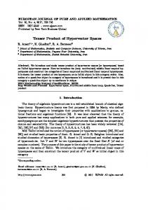
Figure 2: Categorical product
4.3 Categorical product
We nish this section with a note on the relationship between the products we have de ned here and products in category theory (for detailed categorical analyses of products and related operations on predicate transformers we refer to Martin [8] and Naumann [9]). The categorical product of two objects a and b in a category is an object a � b together with a pair of projection morphisms �1 : a � b ! a and �2 : a � b ! b, such that for any object c and morphisms f : c ! a and g : c ! b, there is a unique morphism (f; g) : c ! a � b that satis es the conditions (f; g) ; �1 = f and (f; g) ; �2 = g The categorical product is illustrated in Figure 2. The product f � g : a � b ! a0 � b0 of two morphisms f : a ! a0 and g : b ! b0 is then de ned as follows: f � g = (�1 ; f; �2 ; g) In our framework, state spaces are objects while we consider either state transformers, relations or predicate transformers as morphisms. We generally want the product of two state spaces � and ? to be the cartesian product � � ?. 16
In the category of state transformers the projection functions are de ned by �1: (�; ) = � and �2: (�; ) = . The required unique morphism is given by the pointwise extension of the pairing: (f; g): � =^ (f: �; g: �) and f � g then agrees with our de nition. In the category of relations the projection morphisms are de ned by �1: (�; ): �0 � (� = �0) �2: (�; ): 0 � ( = 0) For P : � ! � ! Bool and Q : � ! ? ! Bool, we de ne (P; Q) : � ! � � ? ! Bool by (P; Q): �: (�; ) =^ P: �: � ^ Q: �: which again makes P � Q agree with our de nition. This gives us a proper product only in the case that P and Q are total relations, i.e., when (8� � 9� � P: �: �) and (8� � 9 � Q: �: ) hold. Hence, the category of total relations does have products in the categorical sense, but the category of relations does not have such products. However, (P; Q) ; �1 � P and (P; Q) ; �2 � Q does hold in general. A category is said to have weak products, if (P; Q) satis es this weaker condition. Hence, we conclude that the category of relations only has weak products, but the subcategory of total relations has ordinary categorical products. The category of predicate transformers is also not equipped with ordinary categorical products. The situation is similar to that for relations; it is possible only to de ne a weak product (as noted in [8]): (S1; S2): q: � =^ (9q1 q2 � q1 � q2 � q ^ S1: q: � ^ S2: q: �) and again S1 � S2 agrees with our de nition. Note that we can de ne it simply as S1 � S2 = h�� � �; �i ; (S1; S2).
4.4 Products with program variables
The predicate transformers that we work with in practical program derivation are statements written in terms of program variables, so it is important to know how products behave in the program variable notation. Assume that x and y are (lists of) program variables and that e and f are (lists of) expressions such that x does not occur free in f and y does not 17
occur free in e. Furthermore assume that x and y are sublists of the disjoint lists u and v, respectively. We can then rewrite a product of assignments to x and y as follows: (var u � x := e) � (var v � y := f ) = fde nition of program variables and assignment notationg (�u � u[x := e]) � (�v � v[y := f ]) = fproduct of state transformersg (�u; v � u[x := e]; v[y := f ]) = fassumptions about x and yg (�u; v � (u; v)[x; y := e; f ]) = fde nition of program variables and assignment notationg (var u; v � x; y := e; f ) From Theorem 6 (c) it then follows that hvar u � x := ei � hvar v � y := f i = (var u; v � x; y := e; f i provided x does not occur free in f and y does not occur free in e. Thus the multiple assignment can be used as a notation for product, i.e., as a parallel assignment to di�erent components. For relational assignments, a similar derivation shows the following: (var u � x := x0 j b) � (var v � y := y0 j c) = (var u; v � x; y := x0; y0 j b ^ c) provided x and x0 do not occur free in c and y and y0 do not occur free in b. Again, Theorem 6 can be used to lift this result to both angelic and demonic assignment statements. We also extend the program variable notation to products, by de ning (var u; v � S � T ) =^ (var u � S ) � (var v � T ) Here u; v stands for a pair of tuples. As an example, we have that (var (x; y); (z; w) � hx := x + yi ; hy := y + 1i � hz := z + wi) = (var x; y � hx := x + yi ; hy := y + 1i) � (var z; w � hz := z + wi)
5 Distributivity properties of products The product operator adds a new construct to the predicate transformer notation. In addition to its intrinsic properties, we also want to know how it interacts with other constructs. In particular, we are interested in studying how the product operator distributes over other operators. 18
5.1 Distributivity over sequential composition
Sequential composition does not in general distribute over products, i.e., (S1 ; S2) � T is di�erent from (S1 � T ) ; (S2 � T ). This is intuitively quite evident, because in the rst case, T is executed only once, but in the second it is executed twice. Product does also not distribute over sequential composition. In fact, this is not even a well-posed question, because T has di�erent type in (S1 � S2); T and in (S1 ; T ) � (S2 ; T ). However, joint distributivity of the form (S1 � S2) ; (T1 � T2) � (S1 ; T1) � (S2 ; T2) is meaningful. In general these two are not equal, as the following simple counterexample shows: (skip � magic) ; (abort � skip) 6= (skip ; abort) � (magic ; skip): According to Theorem 6 and the preemptive properties of magic and abort (see Theorem 9 below), the left hand side is magic while the right hand side is abort. A di�erent counterexample is (skip � [var x � x := x0 j true]) ; (fvar x � x := x0 j trueg � skip) 6= (skip ; fvar x � x := x0 j trueg) � ([var x � x := x0 j true] ; skip) Intuitively speaking, the angel can here take the demon's choice into account when it makes its choice on the left hand side. This is not possible in the right hand side, where the two updates are performed in parallel. These examples indicate that mixing angelic and demonic nondeterminism or miracles and nontermination can cause distributivity to break down. Thus the best we can hope for is that distributivity holds under certain restrictions. However, we rst note that subdistributivity holds generally in one direction. Theorem 7 The re nement (S1 ; T1) � (S2 ; T2) v (S1 � S2) ; (T1 � T2) (1) holds for arbitrary monotonic predicate transformers S1, S2, T1 and T2. Proof We have
(S1 ; T1 � S2 ; T2): q: (�1; �2) � fde nitionsg (9q1 q2 � q1 � q2 � q ^ S1: (T1: q1): �1 ^ S2: (T2: q2): �2) 19
) fmonotonicity of T1 and T2g (9q1 q2 � (T1 � T2): (q1 � q2) � (T1 � T2): q ^ S1: (T1: q1): �1 ^ S2: (T2: q2): �2) ) fTheorem 4g (9q1 q2 � T1: q1 � T2: q2 � (T1 � T2): q ^ S1: (T1: q1): �1 ^ S2: (T2: q2): �2) ) fuse T1: q1 and T2: q2 as existential witnessesg (9q1 q2 � q1 � q2 � (T1 � T2): q ^ S1: q1: �1 ^ S2: q2: �2) � fde nitionsg ((S1 � S2) ; (T1 � T2)): q: (�1; �2) 2
We now show under what restrictions distributivity holds.
Theorem 8 Assume that predicate transformers S1, S2, T1 and T2 are monotonic. Then (S1 ; T1) � (S2 ; T2) = (S1 � S2) ; (T1 � T2) holds if (a) T1 and T2 are universally conjunctive, or
(b) S1 and S2 are strict and T1 and T2 are conjunctive, or (c) S1 and S2 are universally disjunctive, or (d) S1 and S2 are disjunctive and T1 and T2 are terminating. Proof We begin by proving (a). We rst write the predicate transformers
in normal form; S1 = fP1g ; [Q1], T1 = [R1], S2 = fP2g ; [Q2] and T2 = [R2]. Now we show that
fP1g ; [Q1] � fP2g ; [Q2] = (fP1g � fP2g) ; ([Q1] � [Q2]) (* ) First we show re nement: (fP1g � fP2 g) ; ([Q1] � [Q2]): q: (�1; �2) = fde nitionsg (9q1 q2 � q1 � q2 � ([Q1] � [Q2]): q ^ (9 1 � P1 : �1: 1 ^ q1: 1) ^ (9 2 � P2: �2: 2 ^ q2: 2)) 20
= fde nitionsg (9q1 q2 � (8 1 2 � q1: 1 ^ q2: 2 ) (9q10 q20 � q10 � q20 � q ^ Q1: 1 � q10 ^ Q2: 2 � q20 )) ^ (9 1 � P1 : �1: 1 ^ q1: 1) ^ (9 2 � P2: �2: 2 ^ q2: 2)) ) fquanti er rules, use rst conjunct to rewrite restg (9q1 q2 q10 q20 � (8 1 2 � q1: 1 ^ q2: 2 ) q10 � q20 � q ^ Q1: 1 � q10 ^ Q2: 2 � q20 )) ^ (9 1 � P1: �1: 1 ^ Q1: 1 � q10 ) ^ (9 2 � P2: �2: 2 ^ Q2: 2 � q20 )) ) fpredicate calculusg (9q10 q20 � q10 � q20 � q ^ (9 1 � P1: �1: 1 ^ Q1: 1 � q10 ) ^ (9 2 � P2: �2: 2 ^ Q2: 2 � q20 )) = fde nitions of updates and productg (fP1g ; [Q1] � fP2g ; [Q2]): q: (�1; �2) Re nement in the opposite direction follows from Theorem 7. Furthermore, we note the following distributivity property for products of relations: (Q1 � Q2) ; (R1 � R2) = (Q1 ; R1) � (Q2 ; R2) which is straightforward to check. Now we have = = = = =
(S1 � S2) ; (T1 � T2) fde nitionsg (fP1g ; [Q1] � fP2g ; [Q2]) ; ([R1] � [R2]) f(*)g (fP1g � fP2g) ; ([Q1] � [Q2]) ; ([R1] � [R2]) f(**) and Theorem 6g (fP1g � fP2g) ; ([Q1] ; [R1] � [Q2] ; [R2]) f(*)g fP1g ; [Q1] ; [R1] � fP2g ; [Q2] ; [R2] fde nitionsg (S1 ; T1) � (S2 ; T2)
which nishes the proof of (a). 21
(** )
We now prove (b). Again, we rst write the predicate transformers in normal form; S1 = fP1g ; [Q1], T1 = fr1g ; [R1], S2 = fP2g ; [Q2] and T2 = fr2g ; [R2] where [Q1] and [Q2] are strict. Now, = = = = = = = =
(S1 � S2) ; (T1 � T2) fde nitionsg (fP1g ; [Q1] � fP2g ; [Q2]) ; (fr1g ; [R1] � fr2g ; [R2]) f(**), asserts are angelic updatesg (fP1g � fP2g) ; ([Q1] � [Q2]) ; (fr1g � fr2g) ; ([R1] � [R2]) fproduct homomorphism: Theorem 6g (fP1g � fP2g) ; ([Q1] � [Q2]) ; fr1 � r2g ; ([R1] � [R2]) fassert propagation rule S ; fqg = fS: qg ; S (see below)g (fP1g � fP2g) ; f([Q1] � [Q2]): (r1 � r2)g ; ([Q1] � [Q2]) ; ([R1] � [R2]) fTheorem 4, strictnessg (fP1g � fP2g) ; f([Q1]: r1) � ([Q2]: r2)g ; ([Q1] � [Q2]) ; ([R1] � [R2]) fTheorem 6, assert is angelic update, (***)g (fP1g ; f[Q1]: r1g � fP2g ; f[Q2]: r2g) ; ([Q1] ; [R1] � [Q2] ; [R2]) fpart (a)g fP1g ; [Q1] ; fr1g ; [R1] � fP2g ; [Q2] ; fr2g ; [R2] fde nitionsg (S1 ; T1) � (S2 ; T2)
Here we used the assert propagation rule S ; fqg = fS: qg ; S which is easily proved to hold for conjunctive S . Thus the proof of (b) is complete. The proof of (c) is dual to that of (a) and the proof of (d) to that of (b). 2 A consequence of Theorems 8 and 6 is the following homomorphism property of normal forms for monotonic predicate transformers (see Lemma 1 (a))
fP1g ; [Q1] � fP2g ; [Q2] = fP1 � P2g ; [Q1 � Q2]
5.2 Other distributivity properties
The remaining distributivity properties are considerably more straightforward than those for sequential composition.
Theorem 9 Let S and fSi j i 2 I g be monotonic predicate transformers. Then
22
(a) S � magic = magic and magic � S = magic, when S is terminating. (b) S � abort = abort and abort � S = abort. (c) (u i 2 I � Si) � S = (u i 2 I � Si � S ) and S � (u i 2 I � Si) = (u i 2 I � S � Si), when S is conjunctive and I is nonempty. (d) (t i 2 I � Si) � S = (t i 2 I � Si � S ) and S � (t i 2 I � Si) = (t i 2 I � S � Si). Proof For (a) we have
(S � magic): q: (�1; �2) � fde nition of productg (9q1 q2 � q1 � q2 � q ^ S: q1: �1 ^ magic: q2: �2) � fde nition of magic, predicate calculusg (9q1 q2 � q1 � q2 � q ^ S: q1: �1) � f) by monotonicity of �, ( by choosing q2 := falseg (9q1 � q1 � false � q ^ S: q1: �1) � fq1 � false = false, predicate calculusg (9q1 � S: q1: �1) � f) by monotonicity, ( by choosing q1 := trueg S: true: �1 Thus, we have that S � magic = magic, if S: true = true. A symmetric argument shows magic � S = S . Now consider (c), assuming that I is nonempty and S and all Si are conjunctive. Then (u i 2 I � Si � S ): p: (�; �0) � fde nition of meetg (8i 2 I � (Si � S ): p: (�; �0)) � fde nition of productg (8i 2 I � 9q q0 � q � q0 � p ^ Si: q: � ^ S: q0: �0) � fSkolemizationg (9q q0 � 8i 2 I � q: i � q0: i � p ^ Si: (q: i): � ^ S: (q0: i): �0) ) fconjunctivityg (9q q0 � 8i 2 I � q: i � q0: i � p ^ Si: (\ i 2 I � q: i): � ^ S: (\ i 2 I � q0: i): �0) 23
) fchoose q = (\ i 2 I � qi) and q0 = (\ i 2 I � qi0)g (9q q0 � 8i 2 I � q � q0 � p ^ Si: q: � ^ S: q0: �0) � fI nonemptyg (9q q0 � q � q0 � p ^ (8i 2 I � Si: q: �) ^ S: q0: �0) � fde nition of meet and productg ((u i 2 I � Si) � S ): p: (�; �0) which proves (u i 2 I � Si � S ) v (u i 2 I � Si) � S . Re nement in the opposite direction is proved as follows: (u i 2 I � Si) � S v (u i 2 I � Si � S ) ( fde nition of meetg (8i 2 I � (u i 2 I � Si) � S v Si � S ) � fTheorem 5, property of meetg T
The proof of (b) is similar to that of (a) while the proof of (d) is similar to that of (c). 2 To see that the termination condition is required in Theorem 9 (a), consider that abort � magic = abort by (b). The same example shows that the index set cannot be empty in (c), since abort is the empty meet. To see that conjunctivity is required in (c), we note that (hx := 1i � (hy := 1i t hy := 2i) u (hx := 2i � (hy := 1i t hy := 2i) always establishes postcondition x = y, while (hx := 1i u hx := 2i) � (hy := 1i t hy := 2i) does not. For meet and join, we do not have the same kind of joint distributivity as we have for sequential composition. A counterexample is the following: (skip � y := y + 1) u (x := x + 1 � skip) 6= (skip u x := x + 1) � (y := y + 1 u skip) This is because the rst statement must either leave x or y unchanged, while the second statement may change both x and y. Similarly, we have that (skip � y := y + 1) t (x := x + 1 � skip) 6= (skip t x := x + 1) � (y := y + 1 t skip) because in the rst statement, we cannot choose to leave both x and y unchanged, while in the second we can. 24
5.3 Application: data re nement
We illustrate the distributivity properties by applying them to data re nement. Data re nement can on an abstract level be described as a commutativity property: we say that S is data re ned through D by S 0 if the following condition holds: D ; S v S0 ; D where D : Ptran(�0; �) (the decoding), S : Ptran(�; �) (the abstract statement) and S 0 : Ptran(�0 ; �0) (the concrete statement) are monotonic predicate transformers. We talk about 1. general data re nement if D is strict, 2. forward data re nement if D is universally disjunctive, and 3. backward data re nement if D is universally conjunctive and strict More details about the concepts of data re nement (including soundness arguments for general, forward and backward data re nement) can be found elsewhere [7, 10]. Here we concentrate on the algebraic interaction between products and data re nement. Our main question is the following: can the components of a product be data re ned independently of each other? More speci cally, we assume that a product S1 � S2 : Ptran(� � ?; � � ?) and a decoding D are given, so that S1 is data re ned through D by some S10 . The question is now whether S1 � S2 is data re ned through D � skip by S10 � S2. The desired derivation is of the following form: (D � skip) ; (S1 � S2) = f(*)g (D ; S1) � (skip ; S2) v fassumption, skip is identityg (S10 ; D) � (S2 ; skip) v fTheorem 7g (S10 � S2) ; (D � skip) Here the rst justi cation (marked with an asterisk) refers to Theorem 8; thus we have the following four acceptable situations: (a) S1 and S2 are universally conjunctive, (b) D is strict and S1 and S2 are conjunctive 25
(c) D is universally disjunctive (d) D are disjunctive and S1 and S2 are terminating. Cases (a) and (d) place undesired restrictions on S1 and S2 (they must be terminating, which means we cannot work with assertions, loops or other potentially nonterminating constructs). Thus we are left with cases (b) and (c). They show that independent data re nement is possible in a product as follows: 1. general data re nement for conjunctive predicate transformers, and 2. forward data re nement for arbitrary monotonic predicate transformers The negative result is thus that independent backward data re nement of nonconjunctive predicate transformers is not generally possible. This agrees with earlier results indicating that forward data re nement is a generally useful method while backward data re nement can only be used in special circumstances [7, 10].
6 Extension We now consider a special case of product: extending a state predicate, transformer or relation to a larger state space. Consider the predicate p : � ! Bool. We can extend this to a predicate p � true : � � � ! Bool on a state space with new components �. This extension is trivial in the sense that (p � true): (�; �) � p: �, i.e., the truth of the predicate depends only on the original state component �. In a similar way, we can extend a state function f : � ! ? with new state components by taking the product with the unit element, to get f � id : � � � ! ? � �. In this case, we have that (f � id): (�; �) = (f: �; �), i.e, the state transformer leaves the new state component unchanged. This extension is also trivial in the sense that the new state component does not in uence the value of the old component, nor is the new state component changed in the transformation. Finally, for state relations, the extension of R : � ! ? ! Bool is R � Id : � � � ! ? � � ! Bool, where (R � Id): (�; �): ( ; �0) � R: �: ^ � = �0. Thus, again we have that the new state component is left unchanged and does not in uence the resulting value of the old component. 26
6.1 Extension of predicate transformers
Now consider a predicate transformer S : Ptran(�; ?). Exactly as for predicates, functions and relations, we extend this predicate transformer to a larger state space by forming the product with the identity. Thus, the extended predicate transformer is S � skip : Ptran(� � �; ? � �) Exactly as for functions, the extended predicate transformer leaves the added state component � unchanged. The properties of the extension follow from the homomorphism properties of the product.
Corollary 10 The following replacement property holds for extension: (a) S v S 0 � S � skip v S 0 � skip Furthermore, the following distributivity properties generally hold:
(b) abort � skip = abort (c) magic � skip = magic (d) (S u S 0) � skip = (S � skip) u (S 0 � skip) (e) (S t S 0) � skip = (S � skip) t (S 0 � skip) Finally, the following properties hold: (f) skip � skip = skip (g) (S ; S 0) � skip = (S � skip) ; (S 0 � skip) Note that since we have in (a) an equivalence rather than only an implication, and since extension is injective, extension is a homomorphic embedding of Ptran(�; ?) into Ptran(� � �; ? � �). Furthermore, (b){(g) show that extension is a lattice homomorphism and a functor. The fact that extension is a homomorphic embedding means that for any predicate transformer S in Ptran(�; ?), there is a copy S � skip of this predicate transformer in Ptran(� � �; ? � �). A property holds for the copy if and only if it holds for the original predicate transformer, when state spaces are adjusted appropriately. In practical program derivations, we usually take this property for granted and use it without further mentioning. Thus, we may prove a property for 27
some predicate transformer, and then use the property for a copy of the predicate transformer that is de ned for an extended state space. If needed, such a derivation step can always be justi ed by an explicit application of the homomorphism and functor properties of extension. We can use the de nition of extension to compute the weakest precondition predicate transformer for extension. We have that (S � skip): q: (�1; �2) � S: (�� � q: (�; �2)): �1 as shown by the following derivation: (S � skip): q: (�1; �2) � fde nition of product and skipg (9p1 p2 � p1 � p2 � q ^ S: p1: �1 ^ p2 : �2) � fmutual implicationg � (9p1 p2 � p1 � p2 � q ^ S: p1: �1 ^ p2: �2) ) fp1 � p2 � q and p2: �2 imply p1 � (�� � q: (�; �2))g S: (�� � q: (�; �2)): �1 � (9p1 p2 � p1 � p2 � q ^ S: p1: �1 ^ p2: �2) ( f9-introduction, p1 := (�� � q: (�; �2)) and p2 := (�� � � = �2)g S: (�� � q: (�; �2)): �1 � S: (�� � q: (�; �2)): �1 This shows how extension can be de ned without reference to products on the level of predicates or predicate transformers. As a direct consequence, we have (S � skip): (q � true): (�1; �2) � S: q: �1
6.2 Extending by merging and splitting
In an extension the new state components are added at the end of the old ones. In practice, we need more exibility, because the original state components may be merged with the new state components in an arbitrary way, they need not all be collected at the end of the state space as in an extension. Let u be a list of variables that are merged with another list of variables w. Assume that these two lists of variables are disjoint. Let the resulting list be v. For instance, we might merge the variables a : Nat; c : Bool with the variables b : Nat; d : Nat to produce the list a : Nat; b : Nat; c : Bool; d : Nat. Any such merge can described by a merge function � = (�u; w � v) 28
In our example, the merge is described by the function
� = (�(a; c); (b; d) � a; b; c; d) Thus, a merge combines two lists of program variables so that the result is a permutation of the concatenation of the two original lists. The inverse of a merge function is a split function �?1 = (�v � u; w) which splits the merged lists into two lists. It is easily seen that these two operations are inverses, i.e., � ; �?1 = id and �?1 ; � = id. In our example, the split function is �?1 = (�a; b; c; d � (a; c); (b; d)) The extension of state function f : � ! � to a function f 0 : ? ! ? is in the general case now expressed as follows: f 0 = �?1 ; (f � id) ; � In other words, we rst split the state components into old and new components, then we apply the original state function to the rst component and the identity function to the new, and nally we merge the two state partitions together again. As an example, we extend the state function f = (�y : Nat � y + 1) by adding new rst and last state components. We have the merge and split functions � = (�y; (x; b) � x; y; b) �?1 = (�x; y; b � y; (x; b)) and the extended function is f 0 = �?1 ; (f � id) ; � = (�x; y; b � x; y + 1; b) The second identity is calculated using the de nitions of product and composition and a sequence of -reductions. To simplify the notation, we can introduce an extension operation ext which takes a state function (or state relation, predicate transformer) on the old state space and constructs a corresponding extended entity. Thus we de ne extf : �: f = �?1 ; (f � id) ; � 29
State relations are handled in the same way. Thus R : � ! � ! Bool is extended to ? ! ? ! Bool as follows, where ? is again a merge of the components in � and �: extr: �: R = j�?1 j ; (R � Id) ; j�j where jf j is the function f turned into a relation: jf j: �: � ( = f: �). Extension is simpler for state predicates, because the new state component can be discarded altogether. Predicate p : � ! Bool is extended to ? ! Bool, where ? is a merge of the components of � and �, as extp: �: p = �?1 ; (p � true) General extension for predicate transformers is now straightforward. For a given merge function � : � � � ! ?, we de ne the extension of predicate transformer S : Ptran(�; �) to Ptran(?; ?) to be exts: �: S = h�?1 i ; (S � skip) ; h�i The idea is exactly the same here as in the previous extensions. It is easily shown that extension preserves the syntactical structure of state predicates, functions and relations. Theorem 11 Any extension of state predicates, functions, relations and predicate transformers is an order embedding, a lattice homomorphisms and a functor. Proof The proof involves only trivial rewriting and -reductions. For example, we have to show (for predicates) that arbitrary extension of false yields false. We have (extp: �: false): � = fde nition of extensiong (�?1 ; (false � true)): � = fde nition of compositiong (false � true): (�?1: �) = ffalse � true = falseg F
The other proofs are similar, though longer. 2 Because extension is also an injection, it is in fact a homomorphic embedding, both for state predicates, state functions, state relations and predicate transformers. 30
Theorem 11 says that the extension operation preserves all the structure and all properties of the term that is being extended. For instance, if we have proved that P ; Q � R, then P 0 ; Q0 � R0 holds for any extensions P 0, Q0 and R0 of relations P , Q and R (as long as each relation is extended in the same way). This means that we can always lift a result that we have proved for a certain state space to an extended state space, by extending each term in the same way.
6.3 Extension and program variables
Program variables and the assignment notation makes it particularly easy to describe extensions. We begin by illustrating this with an example. Consider the state function (�x; z : Nat � z := x + z). Assume that we want to extend this to a state transformer on the state space x; y; z; w with four components. The new components are also assumed to be natural numbers. Then the merge is described by the function � = (�(x; z); (y; w) � x; y; z; w). The extension is easily computed as
�?1 ; ((var x; z � z := x + z) � id) ; � = (var x; y; z; w � z := x + z) In other words, when the assignment notation is used, extension is just adding new program variables to the list of old program variables. This holds in general, for all kinds of extensions. Moreover, we are also free to reorder the program variables in an extension, and the result is still an extension. By the previous results, we also know that any property that we prove for a state transformer (state relation, predicate transformer) is also true of any extension of it. Hence, we may prove a property for the simple case with no super uous variables, and then infer, whenever needed, that the result also holds for any extension. The fact that the statement notation for predicate transformers is insensitive to extension can be expressed formally, as follows. Theorem 12 Assume that (var u � s) is a statement and that v is a list of variables with u � v. Then there exists a merge function � such that (var v � s) = exts: �: (var u � s) Proof We prove the result for the merge function � = (�u; w � v ), where
w is a list containing all variables that are in v but not in u. The proof is by induction on the structure of the statement s. We show two nontrivial 31
cases: demonic update and sequential composition. For demonic update, we may assume that the statement has the form (var u � [u := u0 j b]) where we without loss of generality can assume that neither w nor w0 occur free in b. Then exts: (�u; w � v ): (var u � [u := u0 j b]) = fde nitionsg h�v � u; wi ; ([�u � �u0 � b] � skip) ; h�u; w � vi = frewrite extensiong h�v � u; wi ; [�u; w � �u0; w0 � b ^ w0 = w] ; h�u; w � vi = fgeneral rule hf i ; [R] ; hf ?1 i = [�� � ��0 � R: (f: �): (f: �0)]g [�v � �v0 � b ^ w0 = w] = fde nitionsg (var v � [u := u0 j b]) For sequential composition, the induction assumption is that both exts: (�u; w � v): (var u � s1) = (var v � s1) and exts: (�u; w � v): (var u � s2) = (var v � s2). We have exts: (�u; w � v ): (var u � s1 ; s2 ) = fde nitionsg h�v � u; wi ; (var u; w � (s1 ; s2) � skip) ; h�u; w � vi = fCorollary 10 (g)g h�v � u; wi ; (var u; w � (s1 � skip) ; (s2 � skip)) ; h�u; w � vi = fadd intermediate split and merge; �?1 ; � = idg h�v � u; wi ; (var u; w � s1 � skip) ; h�u; w � vi ; h�v � u; wi ; (var u; w � s2 � skip) ; h�u; w � vi = fde nitionsg (exts: (�u; w � v): (var u � s1)) ; (exts: (�u; w � v): (var u � s1)) = finduction assumptiong (var v � s1) ; (var v � s2) = fde nitiong (var v � s1 ; s2)
2
A direct consequence of Theorem 12 is (because of Theorem 11) the following. To prove a general property of a statement (var u � s), we can choose any suitable variable environment u (in particular, we can chose u minimal) and the result will then hold for all legal variable environments. 32
7 Extension and product We de ned extension in terms of products. In this section we study the other possibility, i.e., whether products can be de ned in terms of extensions. As we have shown above, extension can be de ned directly as a predicate transformer: (S � skip): q = (��1; �2 � S: (�� � q: (�; �2)): �1) Theorem 8 answers our question for some cases directly. For instance, if S is strict and T is conjunctive, then (S � skip) ; (skip � T ) = (S � T ) = (skip � T ) ; (S � skip) holds. This shows that in certain special cases, independent predicate transformers can be commuted or even combined into a single parallel predicate transformer.
7.1 Products of conjunctive predicate transformers The most important special case are the conjunctive predicate transformers, which are the domain of traditional speci cations and programs. In this case Theorem 8 does not help. However, it turns out that in the conjunctive case we can express the product in terms of extension.
Theorem 13 Assume that S and T are conjunctive predicate transformers. Then
S � T = (S � skip) ; (skip � T ) u (skip � T ) ; (S � skip) Proof Since S and T are assumed to be conjunctive, we can write them in
normal forms, S = fpg ; [P ] and T = fqg ; [Q]. Then
(fpg ; [P ] � skip) ; (skip � fqg ; [Q]) u (skip � fqg ; [Q]) ; (fpg ; [P ] � skip) = fsimilar subderivation for both elements of the meetg 33
� (fpg ; [P ] � skip) ; (skip � fqg ; [Q]) = frewrite skipg (fpg ; [P ] � ftrueg ; [Id]) ; (ftrueg ; [Id] � fqg ; [Q]) = fTheorem 8 (b)g (fpg � ftrueg) ; ([P ] � [Id]) ; (ftrueg � fqg) ; ([Id] � [Q]) = fhomomorphismg fp � trueg ; [P � Id] ; ftrue � qg ; [Id � Q] = fgeneral assertion rule S ; fqg = fS: qg ; S g fp � trueg ; f[P � Id]: (true � q)g ; [P � Id] ; [Id � Q] = fsee separate derivation below (*)g fp � trueg ; f��; �0 � P: � = ; _ q: �0g ; [P � Id] ; [Id � Q] = fhomomorphism, simplifyg f��; �0 � p: � ^ (P: � = ; _ q: �0)g ; [P � Q] � f��; �0 � p: � ^ (P: � = ; _ q: �0)g ; [P � Q] u f��; �0 � (p: � _ Q: �0 = ;) ^ q: �0g ; [P � Q] = fdistributivity, homomorphismg f��; �0 � p: � ^ (P: � = ; _ q: �0) ^ (p: � _ Q: �0 = ;) ^ q: �0g ; [P � Q] = flattice propertiesg f��; �0 � p: � ^ q: �0g ; [P � Q] = fde nition of productg fp � qg ; [P � Q] = fhomomorphismg (fpg � fqg) ; ([P ] � [Q]) = fTheorem 8 (b)g fpg ; [P ] � fqg ; [Q] The subderivation marked (*) is as follows: [P � Id]: (true � q): (�; �0) � fde nition of demonic updateg (8 0 � (P � Id): (�; �0): ( ; 0) ) (true � q): ( ; 0)) � fde nitions of product, Id and trueg (8 0 � P: �: ^ �0 = 0 ) q: 0) � fone-point ruleg (8 � P: �: ) q: �0) � ftautology p ) q � :p _ q, quanti er rulesg (8 � :P: �: ) _ q: �0 34
� fset theoryg (P: � = ;) _ q: �0 2
7.2 Products of monotonic predicate transformers
The following counterexample shows that the characterization in Theorem 13 is not correct in the general case. Assume that � has two components (which we name x and y) and that ? has two components (which we name z and w). We assume that all state components range over types with at least two elements. De ne chaos(x) = [x := x0 j T] choose(x) = fx := x0 j Tg and set S = choose(x) ; chaos(y) T = choose(z) ; chaos(w) 0 S = S � skip T0 = skip � T Then S 0 ; T 0 u T 0 ; S 0 establishes postcondition (�(x; y); (z; w) � z = y _ x = w) but S � T does not. To see this, we rst have
� � ( � � (
(S 0 ; T 0): (�(x; y); (z; w) � z = y): ((x0; y0); (z0; w0)) fde nition of composition, and of S 0 and T 0g (S � skip): ((skip � T ): (�(x; y); (z; w) � z = y)): ((x0; y0); (z0; w0)) fde nition of productg (9p1 p2 � p1 � p2 � (skip � T ): (�(x; y); (z; w) � z = y) ^ S: p1: (x0; y0) ^ p2: (z0; w0)) f9-introduction, S: true = trueg true � true � (skip � T ): (�(x; y ); (z; w) � z = y ) fde nition of product, order on predicatesg (8x y z w � (skip � T ): (�(x; y); (z; w) � z = y): ((x; y); (z; w))) fde nition of product, T g (8x y z w � 9p1 p2 � p1 � p2 � (�(x; y); (z; w) � z = y) ^ p1: (x; y) ^ (9z0 � 8w0 � p2: (z0; w0))) f9-introduction, -reductiong 35
(8x y z w � (�x0; y0 � y0 = y) � (�z0; w0 � z0 = y) � (�(x; y); (z; w) � z = y) ^ y = y ^ (9z0 � z0 = y)) � fsimpli cation, de nition of product of predicatesg (8x y z w x0 y0 z0 w0 � y0 = y ^ z0 = y ) z0 = y0) � fsimpli cationg T
A similar derivation shows (T 0;S 0): (�(x; y); (z; w) � x = w): ((x0; y0); (z0; w0)). By the general rule S: p: � ^ T: q: � ) (S u T ): (p [ q): � these two results give us (S 0 ;T 0uT 0;S 0): (�(x; y); (z; w) � z = y _x = w): (�; ). On the other hand, we have (S � T ): (�(x; y); (z; w) � z = y _ x = w): (�; ) � fde nition of productg (9p1 p2 � p1 � p2 � (�(x; y); (z; w) � z = y _ x = w) ^ S: p1: (x0; y0) ^ T: p2: (z0; w0)) � fde nitionsg (9p1 p2 � (8x y z w � p1: (x; y) ^ p2: (z; w) ) z = y _ x = w) ^ (9x0 � 8y0 � p1: (x0; y0)) ^ (9z0 � 8w0 � p2: (z0; w0)) � fquanti er rulesg (9p1 p2 x0 z0 � (8x y z w � p1: (x; y) ^ p2: (z; w) ) z = y _ x = w) ^ (8y0w0 � p1 : (x0; y0) ^ p2: (z0; w0))) ) freplace in contextg (9p1 p2 x0 z0 � 8y0 w0 � z0 = y0 _ x0 = w0) � fquanti er rulesg (9x0 � 8w0 � x0 = w0) _ (9z0 � 8y0 � z0 = y0) � fcontradiction since variables range over non-singleton typesg F
The fact that the above characterization of products in terms of extension does not work for monotonic predicate transformers in general does not imply that the product of monotonic predicate transformers cannot be expressed in some other way in terms of extension and the usual lattice theoretic operations alone. However, one of the two constructs has to be postulated as 36
fundamental anyway, and taking the product rather than the extension as fundamental is well motivated, as the product has an easy and quite intuitive semantic interpretation.
8 Conclusion Our purpose in this article has been to describe the way in which product state spaces can be handled in a convenient way in the re nement calculus. For this purpose, we have extended higher order logic with special abbreviations that allow us to model program variables and assignment in a simple way. The way we describe program variables here is di�erent from the approach in [5], where a more elaborate mechanism is used. The method for adding program variables that we use here is an example of a shallow embedding of a language (here the program statements) in a logic. This means that the program variable notation is seen as just a syntactic abbreviation. A deep embedding could also be given by introducing program statements s as a new recursive data type, and de ning (var u � s) as a function from this data type to predicate transformers. This would allow us to reason about general properties that all program statements have (e.g., prove that all program statements denote monotonic predicate transformers). The method for handling program variables in [5] is di�erent from both these approaches, as no embedding is used at all. Rather, program variables are de ned in such a way that program statements are directly expressible as predicate transformer terms in the logic. The advantage of the shallow embedding we have given here is that it provides a simple and intuitive notation for program statements on product spaces. The main disadvantage is the one mention above, that reasoning about general properties of program statements has to be done on the metalevel. We have concentrated on the properties of the product operator on product state spaces. The de nition of the product operator that we use here was originally proposed by Naumann [9], and is taken over here directly. Martin [8] approaches predicate transformers di�erently, promoting sums and products from functions to relations and then once more to predicate transformers. The central part of our paper is the detailed analysis of the algebraic properties of the product operator for predicate transformers. As such, it can be seen as a continuation of the corresponding analysis of the algebraic properties of the more traditional operators on predicate transformers that has been done by Back and von Wright in [5]. A small number of basic results noted (and we have pointed out explicitly which ones) in this 37
paper were proved by Back and Butler [2], but they concentrate on a general analysis of di�erent summation and product operators. Our way of treating program variables is combined with the product operator in the extension of predicate transformers to larger state spaces. This is an important and frequently used operation and its regular and simple properties justify the common practice of leaving it implicit in most cases. However, it is important to check that the properties generally assumed do in fact hold, so that we can continue safely to ignore extension in arguments and proofs. The comparison of extension and products shows that for conjunctive predicate transformers, either one of these two operations could be taken as primitive, the other then being de ned in terms of the other. For monotonic predicate transformers in general, we do not presently have this option, thus partly motivating our decision to take products as the primitive operation.
References [1] M. Ainsworth and P.J. Wallis. Co-re nement. Proc. Sixth BCA/FACS Re nement Workshop, London, January 1994. Springer{Verlag. [2] R. Back and M. Butler. Exploring summation and product operations in the re nement calculus. In Mathematics of Program Construction, volume 947 of Lecture Notes in Computer Science, pages 128{158, Kloster Irsee, Germany, July 1995. Springer{Verlag. [3] R. J. Back. Correctness Preserving Program Re nements: Proof Theory and Applications, volume 131 of Mathematical Center Tracts. Mathematical Centre, Amsterdam, 1980. [4] R. J. Back. A calculus of re nements for program derivations. Acta Informatica, 25:593{624, 1988. [5] R. J. Back and J. von Wright. Re nement Calculus: A Systematic Introduction. Springer-Verlag. To appear. [6] E. W. Dijkstra. A Discipline of Programming. Prentice{Hall International, 1976. [7] P. H. Gardiner and C. C. Morgan. A single complete rule for data re nement. Formal Aspects of Computing, 5(4):367{383, 1993. [8] C.E. Martin. Preordered Categories and Predicate Transformers. PhD thesis, Oxford University, 1991. 38
[9] D.A. Naumann. Two-Categories and Program Structure: Data Types, Re nement Calculi and Predicate Transformers. PhD thesis, University of Texas at Austin, 1992. [10] J. von Wright. The lattice of data re nement. Acta Informatica, 31:105{ 135, 1994.
39
Appendix: Additional proofs
Proof of Theorem 3 To prove that the product preserves monotonicity,
assume p � q:
(S1 � S2): p: (�1; �2) � fde nition of productg (9p1 p2 � p1 � p2 � p ^ S1: p1: �1 ^ S2: p2: �2) ) fassumption p � q, transitivityg (9p1 p2 � p1 � p2 � q ^ S1: p1: �1 ^ S2: p2: �2) � fde nition of productg (S1 � S2): q: (�1; �2) For strictness, we have the following derivation: (S1 � S2): false: (�1; �2) � fde nitiong (9q1 q2 � q1 � q2 � false ^ S1: q1: �1 ^ S2: q2: �2) ) fgeneral rule (p � q = false) � (p = false _ q = false)g S1: false: �1 _ S2: false: �2 � fassumed strictnessg F
where we leave the derivation of the rule (p�q = false) � (p = false_q = false) to the reader. Next, product preserves termination: (S1 � S2): true: (�1; �2) � fde nitiong (9q1 q2 � q1 � q2 � true ^ S1: q1: �1 ^ S2: q2: �2) ) ftrue as existential witness for q1 and q2g S1: true: �1 _ S2: true: �2 � fassumed terminationg T
For conjunctivity, we show re nement in the nontrivial direction. The opposite direction follows directly by monotonicity. (\ i 2 I � (S1 � S2): qi): (�1; �2) � fpointwise extensiong 40
(8i 2 I � (S1 � S2): qi: (�1; �2)) � fde nition of productg (8i 2 I � 9p p0 � p � p0 � qi ^ S1: p: �1 ^ S2: p0: �2) � fSkolemisationg (9f g � 8i 2 I � (f: i) � (g: i) � qi ^ S1: (f: i): �1 ^ S2: (g: i): �2) ) fchoose p := (\ i 2 I � f: i), p0 := (\ i 2 I � g: i), conjunctivityg (9p p0 � p � p0 � (\ i 2 I � qi) ^ S1: p: �1 ^ S2: p0: �2) � fde nition of productg (S1 � S2): (\ i 2 I � qi): (�1; �2) Finally, product preserves disjunctivity: (S1 � S2): ([ i 2 I � qi): (�1; �2) � fde nition of productg (9p p0 � p � p0 � ([ i 2 I � qi) ^ S1: p: �1 ^ S2: p0: �2) � fdisjunctivityg (9p p0 � �0 � p: � ^ p0: �0 ^ p � p0 � ([ i 2 I � qi) ^ S1: f�g: �1 ^ S2: f�0g: �2) ) fchoose i so that qi: (�; �0)g (9i 2 I � 9� �0 � f�g � f�0g � qi ^ S1: f�g: �1 ^ S2: f�0g: �2) ) fde nition of productg (9i 2 I � (S1 � S2): qi: (�1; �2)) � fpointwise extensiong ([ i 2 I � (S1 � S2): qi): (�1; �2) and re nement in the opposite direction follows directly by monotonicity.
Proof of Theorem 6 (a) ([p1] � [p2]): q: (�1; �2) � fde nition of productg (9q1 q2 q1 � q2 � q ^ [p1]: q1: �1 ^ [p2]: q2: �2) � fde nition of guardg (9q1 q2 q1 � q2 � q ^ (p1: �1 ) q1: �1) ^ (p2: �2 ) q2: �2)) � fde nition of product of predicatesg (9q1 q2 q1 � q2 � q ^ (p1 � p2): (�1; �2) ) (q1 � q2): (�1; �2)) � f): de nition of order on predicatesg f(: choose q1 := (�� � = �1) and q2 := (�� � = �2)g �
�
�
�
�
41
(p1 � p2): (�1; �2) ) q: (�1; �2) � fde nition of productg [p1 � p2]: q: (�1; �2) The derivation for the assert statement is similar.
Proof of Theorem 6 (b) (fp1g � fp2 g): q: (�1; �2) � fde nition of productg (9q1 q2 q1 � q2 � q ^ fp1 g: q1: �1 ^ fp2g: q2: �2) � fde nition of assertg (9q1 q2 q1 � q2 � q ^ p1 : �1 ^ q1: �1 ^ p2: �2 ^ q2: �2) � fde nition of product of predicatesg (9q1 q2 q1 � q2 � q ^ (p1 � p2 ): (�1; �2) ^ (q1 � q2): (�1; �2)) � f): de nition of order on predicatesg f(: choose q1 := (�� � = �1) and q2 := (�� � = �2)g (p1 � p2): (�1; �2) ^ q: (�1; �2) � fde nition of productg fp1 � p2g: q: (�1; �2) �
�
�
�
�
Proof of Theorem 6 (c) (hf1i � hf2): q: (�1; �2) � fde nition of product of predicate transformersg (9q1 q2 q1 � q2 � q ^ hf1 i: q1: �1 ^ hf2i: q2: �2) � fde nition of functional updateg (9q1 q2 q1 � q2 � q ^ q1: (f1: �1) ^ q2: (f2: �2)) � fde nition of product of predicatesg (9q1 q2 q1 � q2 � q ^ (q1 � q2): (f1: �1; f2: �2)) � f): de nition of order on predicatesg f(: choose q1 := (�� � = �1) and q2 := (�� � = �2)g �
�
�
�
�
q: (f1: �1; f2: �2) � fde nition of product of functionsg q: ((f1 � f2): (�1; �2)) � fde nition of functional updateg hf1 � f2i: q: (�1; �2) 42
Proof of Theorem 6 (e) [R1] � [R2]: q: (�1; �2) � fde nition of product of predicate transformersg (9q1 q2 q1 � q2 � q ^ [R1]: q1: �1 ^ [R2]: q2: �2) � fde nition of demonic updateg (9q1 q2 q1 � q2 � q ^ (8 1 R1: �1: 1 ) q1: 1) ^ (8 2 R2: �2: 2 ) q2: 2)) � fpredicate calculusg (9q1 q2 q1 � q2 � q ^ (8 1 2 R1: �1: 1 ^ R2: �2: 2 ) q1: 1 ^ q2: 2)) � fde nition of product of predicatesg (9q1 q2 q1 � q2 � q ^ (8 1 2 R1: �1: 1 ^ R2: �2: 2 ) (q1 � q2): ( 1; 2)) � f): de nition of order on predicatesg f(: choose q1 := (�� � = �1) and q2 := (�� � = �2)g (9 1 2 R1: �1: 1 ^ R2: �2: 2 ^ q: ( 1; 2)) � fde nition of product of relationsg (9 1 2 (R1 � R2): (�1; �2): ( 1; 2) ^ q: ( 1; 2)) � fde nition of angelic updateg fR1 � R2g: q: (�1; �2) �
�
�
�
�
�
�
�
�
�
�
�
Proof of Theorem 9 (b) (S � abort): q: (�1; �2) � fde nition of product of predicate transformersg (9q1 q2 q1 � q2 � q ^ S1: q1: �1 ^ abort: q2: �2) � fde nition of abortg (9q1 q2 q1 � q2 � q ^ S1: q1: �1 ^ F) � fpredicate calculusg �
�
F
which proves S � abort = abort. A symmetric argument gives abort � S = abort.
Proof of Theorem 9 (d) ((t i 2 I Si) � S ): p: (�; �0) � fde nition of productg �
43
(9q q0 � q � q0 � p ^ ([ i 2 I � Si): q: � ^ S: q0: �0) � fde nition of join, quanti er rulesg (9i 2 I � 9q q0 � q � q0 � p ^ Si: q: � ^ S: q0: �0) � fde nition of productg (9i 2 I � (Si � S ): p: (�; �0)) � fde nition of joing (t i 2 I � Si � S ): p: (�; �0)
44
Turku Centre for Computer Science Lemminkaisenkatu 14 FIN-20520 Turku Finland http://www.tucs.abo.
University of Turku � Department of Mathematical Sciences
� Abo Akademi University � Department of Computer Science � Institute for Advanced Management Systems Research
Turku School of Economics and Business Administration � Institute of Information Systems Science