SUBMITTED TO IEEE TRANSACTIONS ON NEURAL NETWORKS AND LEARNING SYSTEMS 2018
1
Progressive Deep Neural Networks Acceleration via Soft Filter Pruning
arXiv:1808.07471v2 [cs.CV] 24 Aug 2018
Yang He, Xuanyi Dong, Guoliang Kang, Yanwei Fu, and Yi Yang
Abstract—This paper proposed a Progressive Soft Filter Pruning method (PSFP) to prune the filters of deep Neural Networks which can thus be accelerated in the inference. Specifically, the proposed PSFP method prunes the network progressively and enables the pruned filters to be updated when training the model after pruning. PSFP has three advantages over previous works: 1) Larger model capacity. Updating previously pruned filters provides our approach with larger optimization space than fixing the filters to zero. Therefore, the network trained by our method has a larger model capacity to learn from the training data. 2) Less dependence on the pre-trained model. Large capacity enables our method to train from scratch and prune the model simultaneously. In contrast, previous filter pruning methods should be conducted on the basis of the pre-trained model to guarantee their performance. Empirically, PSFP from scratch outperforms the previous filter pruning methods. 3) Pruning the neural network progressively makes the selection of low-norm filters much more stable, which has a potential to get a better performance. Moreover, our approach has been demonstrated effective for many advanced CNN architectures. Notably, on ILSCRC-2012, our method reduces more than 42% FLOPs on ResNet-101 with even 0.2% top-5 accuracy improvement, which has advanced the state-of-the-art. On ResNet-50, our progressive pruning method have 1.08% top-1 accuracy improvement over the pruning method without progressive pruning. Index Terms—Neural Networks, Deep Learning, Computer Vision.
I. I NTRODUCTION ONVOLUTIONAL Neural Networks (CNNs) is increasingly used to structural prediction [1], visual presentation [2], detection [3], eye fixations prediction [4], image saliency computing [5], [6], face recognition [7] and so on. The superior performance of deep CNNs usually comes from the deeper and wider architectures, which cause the prohibitively expensive computation cost. Even if we use more efficient architectures, such as residual connection [8] or inception module [9], it is still difficult in deploying the state-of-the-art CNN models on mobile devices. For example, ResNet-152 has 60.2 million parameters with 231MB storage spaces; besides, it also needs more than 380MB memory footprint and six seconds (11.3 billion float point operations, FLOPs) to process a single image on CPU. The storage, memory, and computation of this cumbersome model significantly exceed the computing limitation of current mobile devices. Therefore, it is essential to maintain the small size of the deep CNN models which has
C
Y. He, X. Dong, G. Kang and Y. Yang are with the Center for AI, University of Technology Sydney, Sydney, NSW 2007, Australia (email:
[email protected];
[email protected];
[email protected];
[email protected].) Y. Fu is with The School of Data Science, Fudan University, Shanghai 200433, China (e-mail:
[email protected].)
Input
Filters
Output
×
Input
Filters
× Pruning
Pruning
Hard pruned never update
Soft pruned allow update
×
× Training
Still zero
Output
Decrease Dimension
× Hard Filter Pruning
Training Non-zero
Stable Dimension
× Soft Filter Pruning
Fig. 1: Hard filter pruning v.s. soft filter pruning. We mark the pruned filter as the orange dashed box. For the hard filter pruning, the pruned filters are always fixed during the whole training procedure. Therefore, the model capacity is reduced and thus harms the performance because the dashed blue box is useless during training. On the contrary, our soft pruning method allows the pruned filters to be updated during the training procedure. In this way, the model capacity is recovered from the pruned model, and thus leads a better accuracy.
relatively low computational cost but high accuracy in realworld applications. Various acceleration methods for the neural network has been proposed [10], [11]. Pruning deep CNNs [12], [13] is an important direction. Recent efforts have been made either on directly deleting some weight values of filters [14] (i.e., weight pruning) or totally discarding some filters (i.e., filter pruning) [15]–[17]. However, the weight pruning may result in the unstructured sparsity of filters, which may still be less efficient in saving the memory usage and computational cost, since the unstructured model cannot leverage the existing high-efficiency BLAS (Basic Linear Algebra Subprograms) libraries. In contrast, the filter pruning enables the model with structured sparsity and more efficient memory usage than weight pruning, and thus takes full advantage of BLAS libraries to achieve a more realistic acceleration. Therefore, the filter pruning is more advocated in accelerating the networks.
SUBMITTED TO IEEE TRANSACTIONS ON NEURAL NETWORKS AND LEARNING SYSTEMS 2018
Nevertheless, most of the previous works on filter pruning still suffer from the problems of 1) the model capacity reduction and 2) the dependence on pre-trained model. Specifically, as shown in Figure 1, most previous works conduct the “hard filter pruning”, which directly delete the pruned filters. The discarded filters will reduce the model capacity of original models, and thus inevitably harm the performance. Moreover, to maintain a reasonable performance with respect to the full models, previous works [15]–[17] always fine-tuned the hard pruned model after pruning the filters of a pre-trained model, which however has low training efficiency and often requires much more training time than the traditional training schema. To address the above mentioned two problems, we propose a novel Soft Filter Pruning (SFP) approach. The SFP dynamically prunes the filters in a soft manner. Particularly, before first training epoch, the filters of almost all layers with small `2 -norm are selected and set to zero. Then the training data is used to update the pruned model. Before the next training epoch, our SFP will prune a new set of filters of small `2 norm. These training processes are continued until converged. Finally, some filters will be selected and pruned without further updating. The SFP algorithm enables the compressed network to have a larger model capacity, and thus achieve a higher accuracy than others. Intuitively, for the pre-trained network, all the filter of the model have information of the training set, some of them are important, and others are not that important thus could be pruned. If we directly prune a large number of filters at the early epoch, some informative filters might not be recovered by retraining even if we use the soft pruning approach. This is because there exist some filters with similar `2 -norm in the neural network, which makes it difficult to choose the right filters to be pruned. Therefore, we propose to prune the network progressively, i.e., small pruning rate at the early epochs, and large pruning rate at later epochs, which is called progressive soft filter pruning (PSFP). In this way, after pruning a small number of filters at the early epochs and retraining the model, the distribution of `2 -norm of the filters would become different, and the information of training set would concentrate on some important filters. In the meantime, less informative filters are much easy to be recognized. In this situation, if we use a larger pruning rate at a later epoch, it is easy to select the unimportant filters because they are becoming discriminative and it is less possible to choose the wrong filters. Contributions. We highlight four contributions: (1) We propose a soft pruning manner to allow the pruned filters to be updated during the training procedure. This soft manner can dramatically maintain the model capacity and thus achieves the superior performance. (2) Our acceleration approach can train a model from scratch and achieve better performance compared to the state-of-the-art. In this way, the fine-tuning procedure and the overall training time is saved. Moreover, using the pre-trained model can further enhance the performance of our approach to advance the state-of-the-art in model acceleration. (3) To reduce the possibility of pruning the wrong filters, we propose to prune the network progressively, i.e., small
2
pruning rate at early epochs and large pruning rate at later epochs. In this way, the filters with less information (in other words, less norm) become distinct after pruning and retraining at early epochs and it is less possible to prune the wrong filters at later epochs if we use a large pruning rate. (4) The extensive experiment on three benchmark datasets demonstrates the effectiveness and efficiency of our PSFP. We accelerate ResNet-110 by two times with about 4% relative accuracy improvement on CIFAR-10, and also achieve state-of-the-art results on ILSVRC-2012.
II. R ELATED W ORKS Most previous works on accelerating CNNs can be roughly divided into three categories, namely, matrix decomposition, low-precision weights, and pruning. In particular, the matrix decomposition of deep CNN tensors is approximated by the product of two low-rank matrices [18]–[22]. This can save the computational cost. Some works [23], [24] focus on compressing the CNNs by using low-precision weights. Pruningbased approaches aim to remove the unnecessary connections of the neural network [14], [15]. Essentially, the work of this paper is based on the idea of pruning techniques; and the approaches of matrix decomposition and low-precision weights are orthogonal but potentially useful here – it may be still worth simplifying the weight matrix after pruning filters, which would be taken as future work. A. Matrix Decomposition. To reduce the computation costs of the convolutional layers, past works have proposed to representing the weight matrix of the convolutional network as a low-rank product of two smaller matrices [18]–[21], [25]. Then the calculation of production of one large matrix turns to the production of two smaller matrices. However, the computation cost of tensor decomposition operation is large, which is not friendly to the training of neural network. In addition, there exists increasing usage of 1 × 1 convolution kernel in some recent neural network, such as the bottleneck building block structure of ResNet [8], which is difficult for matrix decomposition. B. Low Precision. Some other researchers focus on low-precision implementation to compress and accelerate CNN models [23], [24], [26]–[28]. Han [26] proposed to prune the connections of the neural network, and then fine-tuned networks to recover the accuracy drop, after which he quantify the weights to reduce the number of bits of the parameters of a single layer to 5. Zhou [23] proposes trained ternary quantization (TTQ), a method that can reduce the precision of weights in neural networks to ternary values. In [24], the authors present incremental network quantization (INQ), a novel method targeting to efficiently convert pre-trained full-precision CNN model into a low-precision version whose weights are constrained to be either power of two or zero. Under this situation, only low-precision weights are stored and used to inference, thus the storage and computation cost are dramatically reduced.
SUBMITTED TO IEEE TRANSACTIONS ON NEURAL NETWORKS AND LEARNING SYSTEMS 2018
C. Weight Pruning. Many recent works [14], [26], [29] pruning weights of neural network resulting in small models. For example, [14] proposed an iterative weight pruning method by discarding the small weights whose values are below the threshold. [29] proposed the dynamic network surgery to reduce the training iteration while maintaining a good prediction accuracy. [30], [31] leveraged the sparsity property of feature maps or weight parameters to accelerate the CNN models. However, pruning weights always leads to unstructured models, so the model cannot leverage the existing efficient BLAS libraries in practice. Therefore, it is difficult for weight pruning to achieve realistic speedup. D. Filter Pruning. Concurrently with our work, some filter pruning strategies [15]–[17], [32] have been explored. Pruning the filters leads to the removal of the corresponding feature maps. This not only reduces the storage usage on devices but also decreases the memory footprint consumption to accelerate the inference. [15] uses `1 -norm to select unimportant filters and explores the sensitivity of layers for filter pruning. [32] introduces `1 regularization on the scaling factors in batch normalization (BN) layers as a penalty term, and prune channel with small scaling factors in BN layers. [33] proposes a Taylor expansion based pruning criterion to approximate the change in the cost function induced by pruning. [17] adopts the statistics information from next layer to guide the importance evaluation of filters. [16] proposes a LASSO-based channel selection strategy, and a least square reconstruction algorithm to prune filers. However, for all these filter pruning methods, the representative capacity of neural network after pruning is seriously affected by smaller optimization space. E. Discussion. To the best of our knowledge, there is only one approach that uses the soft manner to prune weights [29]. We would like to highlight our advantages compared to this approach as below: 1) Our pruning algorithm focuses on the filter pruning, but they focus on the weight pruning. As discussed above, weight pruning approaches lack the practical implementations to achieve the realistic acceleration. 2) [29] paid more attention to the model compression, whereas our approach can achieve both compression and acceleration of the model. 3) Extensive experiments have been conducted to validate the effectiveness of our proposed approach both on large-scale datasets and the state-of-the-art CNN models. In contrast, [29] only had the experiments on Alexnet which is more redundant than the advanced models, such as ResNet. III. M ETHODOLOGY A. Preliminary We will formally introduce the symbol and annotations in this section. The deep CNN network can be parameterized by {W(i) ∈ RNi+1 ×Ni ×K×K , 1 ≤ i ≤ L} 1 . W(i) denotes 1 Fully-connected
layers can be viewed as convolutional layers with k = 1
3
a matrix of connection weights in the i-th layer. Ni denotes the number of input channels for the i-th convolution layer. L denotes the number of layers. The shapes of input tensor U and output tensor V are Ni ×Hi ×Wi and Ni+1 ×Hi+1 ×Wi+1 , respectively. The convolutional operation of the i-th layer can be written as: Vi,j = Fi,j ∗ U for 1 ≤ j ≤ Ni+1 ,
(1)
where Fi,j ∈ RNi ×K×K represents the j-th filter of the ith layer. W(i) consists of {Fi,j , 1 ≤ j ≤ Ni+1 }. The Vi,j represents the j-th output feature map of the i-th layer. Pruning filters can remove the output feature maps. In this way, the computational cost of the neural network will reduce remarkably. Let us assume the pruning rate is Pi for the i-th layer. The number of filters of this layer will be reduced from Ni+1 to Ni+1 (1 − Pi ), thereby the size of the output tensor Vi,j can be reduced to Ni+1 (1 − Pi ) × Hi+1 × Wi+1 . As the output tensor of i-th layer is the input tensor of i + 1-th layer, we can reduce the input size of i-th layer to achieve a higher acceleration ratio. B. Pruning with hard manner Most of previous filter pruning works [15]–[17], [32] compressed the deep CNNs in a hard manner. We call them as the hard filter pruning (HFP). Typically, these algorithms firstly prune filters of a single layer of a pre-trained model and fine-tune the pruned model to complement the degrade of the performance. Then they prune the next layer and fine-tune the model again until the last layer of the model is pruned. However, once filters are pruned, these approaches will not update these filters again. Therefore, the model capacity is drastically reduced due to the removed filters; and such a hard pruning manner negatively affects the performance of the compressed models. The process of hard filter pruning is shown in the first row of Figure 2. First, some of the filters with small `p -norm (marked in blue) are select and pruned. After retraining, the pruned filters are not able to be updated again thus the `p norm of these pruned filters will be zero during all the training epochs. Besides, the remaining filters (marked in green) might be updated to another value after retraining to make up for the performance degradation due to pruning, which is represented as the first and third filter in HFP-b and HFP-c of Figure 2. After several epochs of retraining to converge the model, a compact model is obtained to accelerate the inference. C. Pruning with soft manner As summarized in Algorithm 1, SFP can dynamically remove the filters in a soft manner. Specifically, the key is to keep updating the pruned filters in the training stage. Such an updating manner brings several benefits. It not only keeps the model capacity of the compressed deep CNN models as the original models, but also avoid the greedy layer by layer pruning procedure and enable pruning almost all layers at the same time. More specifically, SFP can prune a model either in the process of training from scratch, or a pre-trained model. In
SUBMITTED TO IEEE TRANSACTIONS ON NEURAL NETWORKS AND LEARNING SYSTEMS 2018
k-th training epoch filters
‖•‖p
Pruned model
importance
filters
1.231
‖•‖p
2.056
Filter Pruning
0.275
0
1.572
1.572
filters
1.231
0.256
‖•‖p
(k+1)-th training epoch filters
2.512 1.324
2.056
1.572
1.572
0.056
Reconstruction
0.897
3.742
SFP-b
SFP-c
Pruned model filters
1.231
‖•‖p
importance
0 0
importance
‖•‖p
1.231
0.275
k-th training epoch
PSFP-a
0
importance
Filter Pruning
SFP-a ‖•‖p
1.634
Retraining
HFP-c
0.331
filters
0
Pruned model
importance
importance 2.357
HFP-b
2.056
‖•‖p
0
k-th training epoch
‖•‖p
filters
1.231
HFP-a filters
(k+1)-th training epoch
importance
0.331 2.056
4
(k+1)-th training epoch
importance
filters
‖•‖p
importance
1.231
2.512
0.331
0.734
1.324
2.056
2.056
Filter Pruning
0.575
0.575
1.572
1.572
PSFP-b
0.056
Reconstruction
0.897
3.742
PSFP-c
Fig. 2: Overview of HFP (hard filter pruning, first row), SFP (hard filter pruning, second row) and PSFP (progressive filter pruning, third row) (best viewed in color). At the end of each training epoch, we prune the filters based on their importance evaluations. The filters are ranked by their `p -norms (purple rectangles) and the small ones (blue circles) are selected to be pruned. For HFP, after filter pruning, the pruned filter would have no chance to come back during retraining process. This is represented by that HFP-b and HFP-c have the same blue filters with zero `p -norm. For SFP, after filter pruning, the model undergoes a reconstruction process where the pruned filters are capable of being reconstructed (i.e. updated from zeros) by the forward-backward process. The number of pruned filters is same during all training epochs, which is showed by that the number of blue filters in SFP-a is the same as the number of blue filters in SFP-c. While for PSFP, the number of pruned filters is increasing progressively during training epochs, which is represented by that PSFP-c has a larger number of blue filters than PSFP-a. (a): filter instantiations before pruning. (b): filter instantiations after pruning. (c): filter instantiations after reconstruction.
each training epoch, the full model is optimized and trained on the training data. After each epoch, the `2 -norm of all filters are computed for each weighted layer and used as the criterion of our filter selection strategy. Then we will prune the selected filters by setting the corresponding filter weights as zero, which is followed by next training epoch. Finally, the original deep CNNs are pruned into a compact and efficient model. The second row of Figure 2 explained the process of SFP. First, some of the filters with small `p -norm (marked in blue) are select and set to zero. During retraining, we allow the pruned filters to be updated. In this way, the pruned filter whose `p -norm equals to zero might become nonzero again due to retraining, which is represented as the second and fourth filter in SFP-b and SFP-c of Figure 2. After
several operations of pruning and reconstruction to converge the model, a compact model is obtained to accelerate the inference. D. Progressive Soft Filter Pruning (PSFP) As all the filters of the pre-trained model have the information of the training set, if we prune a large number of these informative filters, the information of the neural network obtained from training set would dramatically lose. Even if we pruning the filter with the soft manner, it is still difficult for some important filter to recover by retraining. Therefore, we propose to pruning the neural network progressively. Different from the setting in Algorithm 1 that the pruning rate during all retraining epochs equals to the goal pruning rate Pi , we change the pruning rate at each retraining epoch.
SUBMITTED TO IEEE TRANSACTIONS ON NEURAL NETWORKS AND LEARNING SYSTEMS 2018
5
Algorithm 1 Algorithm Description of SFP
Algorithm 2 Algorithm Description of PSFP
Input: training data: X, pruning rate: Pi Input: the model with parameters W = {W(i) , 0 ≤ i ≤ L} Initialize the model parameter W for epoch = 1; epoch ≤ epochmax ; epoch + + do Update the model parameter W based on X for i = 1; i ≤ L; i + + do Calculate the `2 -norm for each filter kFi,j k2 , 1 ≤ j ≤ Ni+1 Zeroize Ni+1 Pi filters by `2 -norm filter selection end for end for Obtain the compact model with parameters W∗ from W Output: The compact model and its parameters W∗
Input: training data: X Input: pruning rate: Pi , pruning rate decay D Input: the model with parameters W = {W(i) , 0 ≤ i ≤ L} Initialize the model parameter W for epoch = 1; epoch ≤ epochmax ; epoch + + do Update the model parameter W based on X for i = 1; i ≤ L; i + + do Calculate the `2 -norm for each filter kFi,j k2 , 1 ≤ j ≤ Ni+1 0 Calculate the pruning rate at this epoch Pi = H(Pi , D, epoch) by function H 0 Zeroize Ni+1 Pi filters by `2 -norm filter selection end for end for Obtain the compact model with parameters W∗ from W Output: The compact model and its parameters W∗
Specifically, we use a small pruning rate at early epochs, and gradually increase the pruning rate as the epoch number increasing until finally, we reach the goal pruning rate Pi at the last epoch of retraining. The details of PSFP is illustratively explained in Algorithm 2. 1) Progressive Filter selection: We use the `p -norm to evaluate the importance of each filter as Eq. (2). In general, the convolutional results of the filter with the smaller `p -norm would lead to relatively lower activation values, and thus have a less numerical impact on the final prediction of deep CNN models. In term of this understanding, such filters of small `p norm will be given high priority of being pruned than those of higher `p -norm: v u Ni K K uX X X p p |Fi,j (n, k1 , k2 )| . (2) kFi,j kp = t n=1 k1 =1 k2 =1
Different form [34] that uses the same pruning rate Pi to select Ni+1 Pi unimportant filters during the whole retraining 0 process, we use different pruning rate Pi at every epoch to 0 select Ni+1 Pi unimportant filters for the i-th weighted layer. 0 The definition of Pi is list as follows: 0
Pi = H(Pi , D, epoch),
(3)
where Pi represents the goal pruning rate for the i-th weighted layer, Parameter D represents the ratio of the total epoch number when pruning rate equals Pi /4, which will be explicitly explained later. Exponential parameter decay is widely used in optimization [35] to achieve a stable result. Similarly, we change the pruning rate exponentially, the equation is as follows: 0
Pi = a × e−k×epoch + b,
(4)
In order to solve three parameters a, k, b of the above 0 exponential equation, three points consists of (epoch, Pi ) pair are needed to solve the equation. Certainly, the first point is (0, 0), which means the pruning rate is zero before the first training epoch. In addition, to achieve the goal pruning rate Pi at the final retraining epoch, the point (epochmax , Pi ) is essential. Now we have to define the third point
(epochmax × D, Pi /4), to solve the equation. This means that when the epoch number is epochmax × D, the pruning rate increase to 1/4 of the goal pruning rate Pi . 0 In this situation, the lowest Ni+1 Pi filters are selected, e.g., the blue filters in Figure 2. In practice, we use the `2 -norm based on the empirical analysis. 0 2) Filter Pruning: We set the value of selected Ni+1 Pi filters to zero (see the filter pruning step in Figure 2). This can temporarily eliminate their contribution to the network output. Nevertheless, in the following training stage, we still allow these selected filters to be updated, in order to keep the representative capacity and the high performance of the model. In the filter pruning step, we simply prune all the weighted layers at the same time. In this way, we can prune each filter in parallel, which would cost negligible computation time. In contrast, the previous filter pruning methods always conduct layer by layer greedy pruning. After pruning filters of one single layer, existing methods always require training to converge the network [16], [17]. This procedure cost much extra computation time, especially when the depth increases. Moreover, we use the same pruning rate for all weighted layers. Therefore, we need only one hyper-parameter Pi = P to balance the acceleration and accuracy. For different epochs, we could calculate the pruning rate with 0 Pi = H(Pi , D, epoch) = H(P, D, epoch). This can avoid the inconvenient hyper-parameter search or the complicated sensitivity analysis [15]. As we allow the pruned filters to be updated, the model has a large model capacity and becomes more flexible and thus can well balance the contribution of each filter to the final prediction. 3) Reconstruction: After the pruning step, we train the network for one epoch to reconstruct the pruned filters. As shown in Figure 2, the pruned filters are updated to non-zero by back-propagation. In this way, the pruned model have the same capacity as the original model during the training. In contrast, hard filter pruning leads to the decrease of feature maps. The reduction of the feature map would dramatically reduce the model capacity, and further harm the performance. Previous pruning methods usually require a pre-trained model
SUBMITTED TO IEEE TRANSACTIONS ON NEURAL NETWORKS AND LEARNING SYSTEMS 2018
E. Computation Complexity Analysis 1) Theoretical speedup analysis: Suppose the filter pruning rate of the ith layer is Pi , which means the Ni+1 ×Pi filters are set to zero and pruned from the layer, and the other Ni+1 × (1 − Pi ) filters remain unchanged, and suppose the size of the input and output feature map of ith layer is Hi × Wi and Hi+1 × Wi+1 . Then after filter pruning, the dimension of useful output feature map of the ith layer decreases from Ni+1 × Hi+1 × Wi+1 to Ni+1 (1 − Pi ) × Hi+1 × Wi+1 . Note that the output of ith layer is the input of (i + 1) th layer. And we further prunes the (i + 1)th layer with a filter pruning rate Pi+1 , then the calculation of (i + 1)th layer is decrease from Ni+2 × Ni+1 × k 2 × Hi+2 × Wi+2 to Ni+2 (1 − Pi+1 ) × Ni+1 (1−Pi )×k 2 ×Hi+2 ×Wi+2 . In other words, a proportion of 1 − (1 − Pi+1 ) × (1 − Pi ) of the original calculation is reduced, which will make the neural network inference much faster. 2) Realistic speedup analysis: In theoretical speedup analysis, other operations such as batch normalization and pooling are negligible comparing to the convolution operations. Therefore, we consider the FLOPs of convolution operations for computation complexity comparison, which is commonly used in previous work [15], [17]. However, reduced FLOPs cannot bring the same level of realistic speedup because nontensor layers (e.g., batch normalization and pooling layers) also need the inference time on GPU [17]. In addition, the limitation of IO delay, buffer switch and efficiency of BLAS libraries also lead to the wide gap between theoretical and realistic speedup ratio. We compare the theoretical and realistic speedup in Section IV-D. IV. E XPERIMENT In this section, we conduct experiments on several benchmark datasets to validate the effectiveness of our acceleration
30 25 Pruning rate (%)
and then fine-tune it. However, as we integrate the pruning step into the normal training schema, our approach can train the model from scratch. Therefore, the fine-tuning stage is no longer necessary for PSFP. As we will show in experiments, the network trained from scratch by PSFP can obtain the competitive results with the one trained from a well-trained model by others. By leveraging the pre-trained model, our PSFP can obtain a much higher performance, and advance the state-of-the-art. 4) Obtaining Compact Model: PSFP iterates over the filter selection, filter pruning and reconstruction steps. After the model gets converged, we can obtain a sparse model containing many “zero filters”. One “zero filter” corresponds to one feature map. The features maps, corresponding to those “zero filters”, will always be zero during the inference procedure. There will be no influence to remove these filters as well as the corresponding feature maps. Specifically, for the pruning rate Pi in the i-th layer, only Ni+1 (1 − Pi ) filters are nonzero and have an effect on the final prediction. Consider pruning the previous layer, the input channel of i-th layer is changed from Ni to Ni (1 − Pi−1 ). We can thus re-build the i-th layer into a smaller one. Finally, a compact model {W∗ (i) ∈ RNi+1 (1−Pi )×Ni (1−Pi−1 )×K×K } is obtained.
6
20 15 10 5
Fit. func: f(x) = 30.000e 0.055x + 30.000 three points to get the function
0 0
50
100 Epoch
150
200
Fig. 3: Progressively changed pruning rate when the goal pruning rate is 30%. Three blue points are the three pairs to generate the function of pruning rate and the solid curve is the exponential pruning rate function.
method. A. Benchmark Datasets and Experimental Setting Our method is evaluated on three benchmarks: MNIST [37], CIFAR-10 [38] and ILSVRC-2012 [39]. The MNIST has a training set of 60,000 examples, and a test set of 10,000 examples. The CIFAR-10 dataset contains 50,000 training images and 10,000 testing images, which are categorized into 10 classes. ILSVRC-2012 is a large-scale dataset containing 1.28 million training images and 50k validation images of 1,000 classes. As discussed in [16], [17], [36], ResNet is less redundancy, and thus more difficult to get accelerated than VGGNet [40]. Therefore, we focus on pruning the challenging ResNet model. In the MNIST experiments, we use the default parameter setting as [37], and use the PyTorch implementation [41] of the network and training schedule. We train the network for 20 epochs to get a more stable result. In the CIFAR-10 experiments, we use the default parameter setting as [42] and follow the training schedule in [43]. For CIFAR-10 dataset, we test our SFP on ResNet-20, 32, 56 and 110. We use several different pruning rates, and also analyze the difference between using the pre-trained model and from scratch. In addition, we test our PSFP on ResNet-56 and 110 with different pruning rate. On ILSVRC-2012, we follow the same parameter settings as [8], [42]. We use the same data argumentation strategies with PyTorch implementation [41]. We test our SFP and PSFP on ResNet-18, 34, 50 and 101; and we use the same pruning rate 30% for all the models. All the convolutional layer of ResNet are pruned with the same pruning rate at the same time. (We do not prune the projection shortcuts for simplification, which only need negligible time and do not affect the overall cost.) For progressive pruning, we set the D in equation 3 as 1/8. For example, if we use the goal pruning rate as 30%, then the pruning rate increases exponentially as shown in figure 3, We conduct our SFP and PSFP operation at the end of every training epoch. For pruning a scratch model, we use the normal training schedule. For pruning a pre-trained model, we reduce
SUBMITTED TO IEEE TRANSACTIONS ON NEURAL NETWORKS AND LEARNING SYSTEMS 2018
7
TABLE I: Comparison of ResNet on Cifar-10. In “Fine-tune?” column, “Y” and “N” indicate whether to use the pre-trained model as initialization or not. The “Accu. Drop” is the accuracy of the pruned model minus that of the baseline model, so negative number means the accelerated model has a higher accuracy than the baseline model. A smaller number of ”Accu. Drop” is better. We run every experiment for three times to get the mean and standard deviation of the accuracy. Depth 20
32
56
110
Method Dong et al. [36] SFP(10%) SFP(20%) SFP(30%) Dong et al. [36] SFP(10%) SFP(20%) SFP(30%) Li et al. [15] Li et al. [15] He et al. [16] He et al. [16] SFP(10%) SFP(20%) SFP(30%) SFP(40%) SFP(30%) SFP(40%) PSFP(30%) PSFP(40%) PSFP(30%) PSFP(40%) Li et al. [15] Li et al. [15] Dong et al. [36] SFP(10%) SFP(20%) SFP(30%) SFP(40%) SFP(30%) SFP(40%) PSFP(10%) PSFP(20%) PSFP(30%) PSFP(40%) PSFP(10%) PSFP(20%) PSFP(30%) PSFP(40%)
Fine-tune? N N N N N N N N N Y N Y N N N N Y Y N N Y Y N Y N N N N N Y Y N N N N Y Y Y Y
Baseline Accu. (%) 91.53 92.20 ± 0.18 92.20 ± 0.18 92.20 ± 0.18 92.33 92.63 ± 0.70 92.63 ± 0.70 92.63 ± 0.70 93.04 93.04 92.80 92.80 93.59 ± 0.58 93.59 ± 0.58 93.59 ± 0.58 93.59 ± 0.58 93.59 ± 0.58 93.59 ± 0.58 93.59 ± 0.58 93.59 ± 0.58 93.59 ± 0.58 93.59 ± 0.58 93.53 93.53 93.63 93.68 ± 0.32 93.68 ± 0.32 93.68 ± 0.32 93.68 ± 0.32 93.68 ± 0.32 93.68 ± 0.32 93.68 ± 0.32 93.68 ± 0.32 93.68 ± 0.32 93.68 ± 0.32 93.68 ± 0.32 93.68 ± 0.32 93.68 ± 0.32 93.68 ± 0.32
Accelerated Accu. (%) 91.43 92.24 ± 0.33 91.20 ± 0.30 90.83 ± 0.31 90.74 93.22 ± 0.09 90.63 ± 0.37 90.08 ± 0.08 91.31 93.06 90.90 91.80 93.89 ± 0.19 93.47 ± 0.24 93.10 ± 0.20 92.26 ± 0.31 93.78 ± 0.22 93.35 ± 0.31 93.05 ± 0.19 92.44 ± 0.07 93.25 ± 0.23 93.12 ± 0.20 92.94 93.30 93.44 93.83 ± 0.19 93.93 ± 0.41 93.38 ± 0.30 92.62 ± 0.60 93.86 ± 0.21 92.90 ± 0.18 93.70 ± 0.55 93.94 ± 0.56 93.29 ± 0.45 93.20 ± 0.10 93.46 ± 0.12 93.38 ± 0.06 93.37 ± 0.12 93.10 ± 0.06
the learning rate by 10 compared to the schedule for the scratch model. We run each experiment three times and report the “mean ± std”. We compare the performance with other stateof-the-art acceleration algorithms [15]–[17], [36]. B. LeNet-5 on MNIST As stated in section III-A, the fully-connected layer can be viewed as the convolutional layer with kernel size k = 1. Suppose the pruning rate for i-th layer is Pi , filter pruning leads to the size of fully-connected layer changes from {W(i) ∈ RNi+1 ×Ni } to {W(i) ∈ RNi+1 (1−Pi )×Ni (1−Pi−1 ) }. In order to test the pruning effect of the algorithm on the fully-connected layer, we pruning the first fully-connected layer of LeNet-5. The baseline accuracy on MNIST is 98.63± 0.04, and the pruning result is shown in Table III. After pruning 30% of the neurons of the fully-connected layer, the accuracy drop is only 0.07%, which means the pruning algorithm works well on the fully-connected layer. We find
Accu. Drop (%) 0.10 -0.04 1.00 1.37 1.59 -0.59 0.00 0.55 1.75 -0.02 1.90 1.00 -0.30 0.12 0.49 1.33 -0.19 0.24 0.54 1.15 0.34 0.47 0.61 0.20 0.19 -0.15 -0.25 0.30 1.04 -0.18 0.78 -0.02 -0.24 0.39 0.48 -0.22 -0.30 0.31 0.58
FLOPs 3.20E7 3.44E7 2.87E7 2.43E7 4.70E7 5.86E7 4.90E7 4.03E7 9.09E7 9.09E7 1.070E8 8.98E7 7.40E7 5.94E7 7.40E7 5.94E7 7.40E7 5.94E7 7.40E7 5.94E7 1.55E8 1.55E8 2.16E8 1.82E8 1.50E8 1.21E8 1.50E8 1.21E8 2.16E8 1.82E8 1.50E8 1.21E8 2.16E8 1.82E8 1.50E8 1.21E8
Pruned FLOPs(%) 20.3 15.2 29.3 42.2 31.2 14.9 28.8 41.5 27.6 27.6 50.0 50.0 14.7 28.4 41.1 52.6 41.1 52.6 41.1 52.6 41.1 52.6 38.6 38.6 34.2 14.6 28.2 40.8 52.3 40.8 52.3 14.6 28.2 40.8 52.3 14.6 28.2 40.8 52.3
that the SFP and PSFP algorithm have a similar result on MNIST. As the previous works on pruning MNIST always pruning ’weight’ of the network instead of the ’filter’ of the network, the comparison results are not listed. C. ResNet on CIFAR-10 Table I shows the results on CIFAR-10. Our SFP could achieve a better performance than the other state-of-the-art hard filter pruning methods. For example, [15] use the hard pruning method to accelerate ResNet-110 by 38.6% speedup ratio with 0.61% accuracy drop when without fine-tuning. When using pre-trained model and fine-tuning, the accuracy drop becomes 0.20%. However, we can accelerate the inference of ResNet-110 to 40.8% speed-up with only 0.30% accuracy drop without fine-tuning. When using the pre-trained model, we can even outperform the original model by 0.18% with about more than 40% FLOPs reduced. PSFP could achieve better performance than SFP when pruning rate is large. For example, when the pruning rate is
SUBMITTED TO IEEE TRANSACTIONS ON NEURAL NETWORKS AND LEARNING SYSTEMS 2018
8
TABLE II: Overall performance of pruning ResNet on ImageNet. In “Fine-tune?” column, “Y” and “N” indicate whether to use the pretrained model as initialization or not. The “Accu. Drop” is the accuracy of the pruned model minus that of the baseline model, so negative number means the accelerated model has a higher accuracy than the baseline model. A smaller number of ”Accu. Drop” is better. We run some ResNet-18 for three times to get the mean and standard deviation of the accuracy. For the other depths of ResNet, we just list the one-view accuracy. Depth
18
34
50
101
Finetune? Dong et al. [36] N SFP(30%) N SFP(30%) Y PSFP(30%) N PSFP(30%) Y Li et al. [15] Y SFP(30%) N SFP(30%) Y PSFP(30%) N PSFP(30%) Y He et al. [16] Y Luo et al. [17] Y SFP(30%) N SFP(30%) Y PSFP(30%) N PSFP(30%) Y SFP(30%) N SFP(30%) Y PSFP(30%) N PSFP(30%) Y Method
Top-1 Accu. Top-1 Accu. Baseline(%) Accelerated(%) 69.98 66.33 70.23±0.06 67.25±0.13 70.23±0.06 60.79 70.23±0.06 67.41 70.23±0.06 68.02 73.23 72.17 73.92 71.83 73.92 72.29 73.92 71.72 73.92 72.53 72.88 72.04 76.15 74.61 76.15 62.14 76.15 74.88 76.15 75.53 77.37 77.03 77.37 77.51 77.37 77.01 77.37 77.28
Top-5 Accu. Top-5 Accu. Baseline(%) Accelerated(%) 89.24 86.94 89.51±0.10 87.76±0.06 89.51±0.10 83.11 89.51±0.10 87.89 89.51±0.10 88.19 91.62 90.33 91.62 90.90 91.62 90.65 91.62 91.04 92.20 90.80 91.14 90.67 92.87 92.06 92.87 84.60 92.87 92.39 92.87 92.73 93.56 93.46 93.56 93.71 93.56 93.43 93.56 93.69
TABLE III: Accuracy of MNIST on LeNet-5 under different pruning rate. Pruning rate(%) Accuracy
10 98.65 ± 0.03
20 98.61 ± 0.05
30 98.55 ± 0.07
40%, PSFP could achieve 93.10% while SFP only achieves 92.90% if we prune the pre-trained model. If we train the model from scratch, PSFP could achieve 93.20% while SFP only achieves 92.62%. When pruning rate is small, we find the performance of SFP and PSFP is competitive. We find that SFP works better for the shallower network, such as ResNet-56, while PSFP works better for the deeper network. These results validate the effectiveness of our SFP and PSFP algorithm which can produce a more compressed model with comparable performance to the original model. D. ResNet on ILSVRC-2012 TABLE IV: Comparison on the theoretical and realistic speedup. We only count the time consumption of the forward procedure. Model ResNet-18 ResNet-34 ResNet-50 ResNet-101
Baseline time (ms) 37.10 63.97 135.01 219.71
Pruned time (ms) 26.97 45.14 94.66 148.64
Realistic Speed-up(%) 27.4 29.4 29.8 32.3
Theoretical Speed-up(%) 41.8 41.1 41.8 42.2
Table II shows that SFP outperforms other state-of-the-art methods. For ResNet-34, SFP without fine-tuning achieves more inference speedup to the hard pruning method [17], but the accuracy of our pruned model exceeds their model by
Top-1 Accu. Drop(%) 3.65 2.98 9.44 2.82 2.21 1.06 2.09 1.63 2.20 1.39 0.84 1.54 14.01 1.27 0.62 0.34 -0.14 0.36 0.09
Top-5 Accu. Drop(%) 2.30 1.75 6.40 1.62 1.32 1.29 0.72 0.97 0.58 1.40 0.47 0.81 8.27 0.48 0.14 0.10 -0.15 0.13 -0.13
Pruned FLOPs(%) 34.6 41.8 41.8 41.8 41.8 24.2 41.1 41.1 41.1 41.1 50.0 36.7 41.8 41.8 41.8 41.8 42.2 42.2 42.2 42.2
2.57%. Moreover, for pruning a pre-trained ResNet-101, SFP reduces more than 40% FLOPs of the model with even 0.2% top-5 accuracy increase, which is the state-of-the-art result. In contrast, the performance degradation is inevitable for hard filter pruning method. Maintained model capacity of SFP is the main reason for the superior performance. In addition, the non-greedy all-layer pruning method may have a better performance than the locally optimal solution obtained from previous greedy pruning method, which seems to be another reason. However, pruning the pre-trained model with SFP algorithm would lead to dramatic accuracy degradation occasionally, which is stated in [34]. For example, when we prune the pre-trained ResNet-18 using SFP, the top-1 accuracy drop is 9.44%. Moreover, if we prune the pre-trained ResNet-50 using SFP, the top-1 accuracy drop is even 14.01%. However, if we use PSFP to prune the model progressively, the top1 accuracy drop of ResNet-18 and ResNet-50 are 2.21% and 0.62%, respectively. On ResNet-50, PSFP could achieve 75.53% top-1 accuracy, which has 1.08% top-1 accuracy improvement over the best result of SFP. On ResNet-50, PSFP could achieve 68.02% top-1 accuracy, which has 0.77% top-1 accuracy improvement over the best result of SFP. On ResNet34 and ResNet-101, the result of PSFP is comparable with SFP algorithm. Therefore, we could achieve a much stable performance if we use PSFP to prune the neural network. The accuracy of the model during training for soft filter pruning method and progressive filter pruning method are shown in the Figure 4. We run this comparison experiment on ResNet-50, with pruning rate 30%. The blue solid line and red dashed line indicate the accuracy of the model before and
SUBMITTED TO IEEE TRANSACTIONS ON NEURAL NETWORKS AND LEARNING SYSTEMS 2018
before pruning after pruning Performance gap
100 50 0 50
0
50 Epoch
before pruning after pruning Performance gap
150 Accuracy (%)
Accuracy (%)
150
100
(a) Soft Filter Pruning
100 50 0 50
0
50 Epoch
100
(b) Progressive Filter Pruning
Fig. 4: The influence of pruning of ResNet-50 on ImageNet regarding different pruning method. The performance gap is calculated by the performance after pruning subtracting that before pruning. TABLE V: Accuracy of CIFAR-10 on ResNet-110 under different pruning rate with different filter selection criteria. Pruning rate(%) `1 -norm `2 -norm
10 93.68 ± 0.60 93.89 ± 0.19
20 93.68 ± 0.76 93.93 ± 0.41
30 93.34 ± 0.12 93.38 ± 0.30
after pruning, respectively. The black line is the performance gap due to pruning, which is calculated by the accuracy after pruning subtracting that before pruning. We find that the performance gap of SFP is not stable for during all the retraining epochs. On the contrary, the performance gap of PSFP is not stable at the early 30 epochs, and become stable afterwards. This is become SFP directly prune a large number of filters, which leads to the loss of a large quantity of pre-trained information of the network, thus the influence of pruning is large and hard to be recovered by retraining. In contrast, PSFP pruned a small number of filters at early epochs, then increase the number of pruned filters at later epochs, this progressive pruning makes the network has time to recover from the information of by retraining, thus stabilizing the pruning process. In order to test the realistic speedup ratio, we measure the forward time of the pruned models on one GTX1080 GPU with a batch size of 64. The results are shown in Table IV. The gap between theoretical and realistic model may come from non-tensor layers and the limitation of IO delay, buffer switch and efficiency of BLAS libraries. E. Ablation Study Extensive ablation study is also conducted to further analyze each component of our model. 1) Filter Selection Criteria: The magnitude based criteria such as `p -norm are widely used to filter selection because computational resources cost is small [15]. We compare the `2 -norm and `1 -norm, and the results are shown in Table V. We find that the performance of `2 -norm criteria is slightly better than that of `1 -norm criteria. The result of `2 -norm is dominated by the largest element, while the result of `1 -norm is also largely affected by other small elements. Therefore, filters with some large weights would be preserved by the `2 norm criteria. Consequently, the corresponding discriminative features are kept so the performance of the pruned model is better.
9
2) Varying pruning rates: To comprehensively understand SFP, we test the accuracy of different pruning rates for ResNet110, shown in Figure 5(a). As the pruning rate increases, the accuracy of the pruned model first rises above the baseline model and then drops approximately linearly. For the pruning rate between 0% and about 23%, the accuracy of the accelerated model is higher than the baseline model. This shows that our SFP has a regularization effect on the neural network because SFP reduces the over-fitting of the model. 3) Sensitivity of SFP interval: By default, we conduct our SFP operation at the end of every training epoch. However, different SFP intervals may lead to different performance; so we explore the sensitivity of SFP interval. We use the ResNet110 under pruning rate 30% as a baseline, and change the SFP interval from one epoch to ten epochs, as shown in Figure 5(b). It is shown that the model accuracy has no large fluctuation along with the different SFP intervals. Moreover, the model accuracy of most (80%) intervals surpasses the accuracy of one epoch interval. Therefore, we can even achieve a better performance if we fine-tune this parameter. 4) Selection of pruned layers: Previous works always prune a portion of the layers of the network. Besides, different layers always have different pruning rates. For example, [15] only prunes insensitive layers, [17] skips the last layer of every block of the ResNet, and [17] prunes more aggressive for shallower layers and prune less for deep layers. Similarly, we compare the performance of pruning first and second layer of all basic blocks of ResNet-110. We set the pruning rate as 30%. The model with all the first layers of blocks pruned has an accuracy of 93.96 ± 0.13%, while the model with all the second layers of blocks pruned has an accuracy of 93.38 ± 0.44%. Therefore, different layers have different sensitivity for SFP. Consequently, careful selection of pruned layers would potentially lead to performance improvement, although more hyper-parameters are needed. 5) Sensitivity of parameter D of PSFP algorithm: We change the parameter D in the Equation 3 to comprehensively understand PSFP, and the results are shown in the Figure 5(c). We use ResNet-56 on CIFAR-10 and set the pruning rate as 40%. When changing the parameter D from 7 to 16, we find the model accuracy has no large fluctuation along with the different parameter D, which shows that the parameter D has little effect on the final result of pruning. V. C ONCLUSION & F UTURE W ORK In this paper, we propose the PSFP, a progressive soft filter pruning approach, to accelerate the deep CNNs. During the training procedure, we prune the filters progressively and allow the pruned filters to be updated. This progressively pruning could make the pruning process more stable and the soft manner could maintain the model capacity and thus achieve the superior performance. Remarkably, without using the pre-trained model, our PSFP can achieve the competitive performance compared to the state-of-the-art approaches. Moreover, by leveraging the pre-trained model, our PSFP achieves a better result and advances the state-of-the-art in the field of model acceleration. The result shows our PSFP
10
93.6
94.0
Baseline Model Accelerated Model 0
10
20
30 40 50 Pruning rate (%)
60
93.4
93.5
Accuracy (%)
94.0 93.5 93.0 92.5 92.0 91.5 91.0
Accuracy (%)
Accuracy (%)
SUBMITTED TO IEEE TRANSACTIONS ON NEURAL NETWORKS AND LEARNING SYSTEMS 2018
93.0 92.5 92.0
2
3
4
93.0 92.8 92.6
Other epochs One epoch 1
93.2
5 6 Epoch
7
8
9
10
92.4
PSFP from pre-trained model PSFP from scratch model 8
10
12 Parameter D
14
16
(a) Accuracy of ResNet-110 on CIFAR-10 re- (b) Accuracy of ResNet-110 on CIFAR-10 regard- (c) Accuracy of ResNet-56 on CIFAR-10 when garding different pruning rates. ing different pruning intervals. pruning rate is 40% regarding different parameter D in the Equation 3.
Fig. 5: Ablation study of SFP and PSFP. (Solid line and shadow denotes the mean and standard deviation of three experiment, respectively.)
have a better performance than the pruning method without progressive pruning. Furthermore, PSFP can be combined with other acceleration algorithms, e.g., matrix decomposition and low-precision weights, to further improve the performance. We will explore this in our future work. R EFERENCES [1] J. Li, X. Mei, D. Prokhorov, and D. Tao, “Deep neural network for structural prediction and lane detection in traffic scene,” IEEE Transactions on Neural Networks and Learning Systems, vol. 28, no. 3, pp. 690–703, 2017. [2] H. Cecotti, M. P. Eckstein, and B. Giesbrecht, “Single-trial classification of event-related potentials in rapid serial visual presentation tasks using supervised spatial filtering,” IEEE Transactions on Neural Networks and Learning Systems, vol. 25, no. 11, pp. 2030–2042, 2014. [3] J. Liu, M. Gong, K. Qin, and P. Zhang, “A deep convolutional coupling network for change detection based on heterogeneous optical and radar images,” IEEE Transactions on Neural Networks and Learning Systems, 2016. [4] N. Liu, J. Han, T. Liu, and X. Li, “Learning to predict eye fixations via multiresolution convolutional neural networks,” IEEE Transactions on Neural Networks and Learning Systems, 2016. [5] T. Chen, L. Lin, L. Liu, X. Luo, and X. Li, “Disc: Deep image saliency computing via progressive representation learning,” IEEE Transactions on Neural Networks and Learning Systems, vol. 27, no. 6, pp. 1135– 1149, 2016. [6] C. Xia, F. Qi, and G. Shi, “Bottom–up visual saliency estimation with deep autoencoder-based sparse reconstruction,” IEEE Transactions on Neural Networks and Learning Systems, vol. 27, no. 6, pp. 1227–1240, 2016. [7] M. Shao, Y. Zhang, and Y. Fu, “Collaborative random faces-guided encoders for pose-invariant face representation learning,” IEEE Transactions on Neural Networks and Learning Systems, vol. 29, no. 4, pp. 1019–1032, 2018. [8] K. He, X. Zhang, S. Ren, and J. Sun, “Deep residual learning for image recognition,” in Proc. IEEE Conf. Comput. Vis. Pattern Recognit. (CVPR), Jun. 2016, pp. 770–778. [9] C. Szegedy, W. Liu, Y. Jia, P. Sermanet, S. Reed, D. Anguelov, D. Erhan, V. Vanhoucke, and A. Rabinovich, “Going deeper with convolutions,” in Proc. IEEE Conf. Comput. Vis. Pattern Recognit. (CVPR), Jun. 2015, pp. 1–9. [10] J. Wang, C. Xu, X. Yang, and J. M. Zurada, “A novel pruning algorithm for smoothing feedforward neural networks based on group lasso method,” IEEE Transactions on Neural Networks and Learning Systems, vol. 29, no. 5, pp. 2012–2024, 2018. [11] L.-W. Kim, “Deepx: Deep learning accelerator for restricted boltzmann machine artificial neural networks,” IEEE Transactions on Neural Networks and Learning Systems, vol. 29, no. 5, pp. 1441–1453, 2018. [12] B. Hassibi and D. G. Stork, “Second order derivatives for network pruning: Optimal brain surgeon,” in Advances in neural information processing systems, 1993, pp. 164–171. [13] R. Reed, “Pruning algorithms-a survey,” IEEE Transactions on Neural Networks, vol. 4, no. 5, pp. 740–747, 1993.
[14] S. Han, J. Pool, J. Tran, and W. Dally, “Learning both weights and connections for efficient neural network,” in Proc. NIPS, 2015, pp. 1135– 1143. [15] H. Li, A. Kadav, I. Durdanovic, H. Samet, and H. P. Graf, “Pruning filters for efficient convnets,” in ICLR, 2017. [16] Y. He, X. Zhang, and J. Sun, “Channel pruning for accelerating very deep neural networks,” in Proc. IEEE Int. Conf. Comput. Vis. (ICCV), Oct. 2017, pp. 1398–1406. [17] J.-H. Luo, J. Wu, and W. Lin, “ThiNet: A filter level pruning method for deep neural network compression,” in Proc. IEEE Int. Conf. Comput. Vis. (ICCV), Oct. 2017, pp. 5068–5076. [18] M. Jaderberg, A. Vedaldi, and A. Zisserman, “Speeding up convolutional neural networks with low rank expansions,” in Proc. BMVC, 2014. [19] X. Zhang, J. Zou, K. He, and J. Sun, “Accelerating very deep convolutional networks for classification and detection,” IEEE Transactions on Pattern Analysis and Machine Intelligence, vol. 38, no. 10, pp. 1943– 1955, 2016. [20] X. Zhang, J. Zou, X. Ming, K. He, and J. Sun, “Efficient and accurate approximations of nonlinear convolutional networks,” in Proc. IEEE Conf. Comput. Vis. Pattern Recognit. (CVPR), 2015, pp. 1984–1992. [21] C. Tai, T. Xiao, Y. Zhang, X. Wang et al., “Convolutional neural networks with low-rank regularization,” in ICLR, 2016. [22] J. Park, S. Li, W. Wen, P. T. P. Tang, H. Li, Y. Chen, and P. Dubey, “Faster cnns with direct sparse convolutions and guided pruning,” in ICLR, 2017. [23] C. Zhu, S. Han, H. Mao, and W. J. Dally, “Trained ternary quantization,” ICLR, 2017. [24] A. Zhou, A. Yao, Y. Guo, L. Xu, and Y. Chen, “Incremental network quantization: Towards lossless cnns with low-precision weights,” ICLR, 2017. [25] J.-T. Chien and Y.-T. Bao, “Tensor-factorized neural networks,” IEEE Transactions on Neural Networks and Learning Systems, vol. 29, no. 5, pp. 1998–2011, 2018. [26] S. Han, H. Mao, and W. J. Dally, “Deep compression: Compressing deep neural networks with pruning, trained quantization and huffman coding,” in ICLR, 2015. [27] I. Hubara, M. Courbariaux, D. Soudry, R. El-Yaniv, and Y. Bengio, “Binarized neural networks,” in Advances in neural information processing systems, 2016, pp. 4107–4115. [28] M. Rastegari, V. Ordonez, J. Redmon, and A. Farhadi, “Xnor-net: Imagenet classification using binary convolutional neural networks,” in European Conference on Computer Vision. Springer, 2016, pp. 525– 542. [29] Y. Guo, A. Yao, and Y. Chen, “Dynamic network surgery for efficient DNNs,” in Proc. NIPS, 2016, pp. 1379–1387. [30] W. Wen, C. Wu, Y. Wang, Y. Chen, and H. Li, “Learning structured sparsity in deep neural networks,” in Proc. NIPS, 2016, pp. 2074–2082. [31] V. Lebedev and V. Lempitsky, “Fast convnets using group-wise brain damage,” in Proc. IEEE Conf. Comput. Vis. Pattern Recognit. (CVPR), 2016, pp. 2554–2564. [32] Z. Liu, J. Li, Z. Shen, G. Huang, S. Yan, and C. Zhang, “Learning efficient convolutional networks through network slimming,” in Proc. IEEE Int. Conf. Comput. Vis. (ICCV), Oct. 2017, pp. 2755–2763. [33] P. Molchanov, S. Tyree, T. Karras, T. Aila, and J. Kautz, “Pruning convolutional neural networks for resource efficient transfer learning,” in ICLR, 2017.
SUBMITTED TO IEEE TRANSACTIONS ON NEURAL NETWORKS AND LEARNING SYSTEMS 2018
[34] Y. He, G. Kang, X. Dong, Y. Fu, and Y. Yang, “Soft filter pruning for accelerating deep convolutional neural networks,” in International Joint Conference on Artificial Intelligence, 2018. [35] D. P. Kingma and J. Ba, “Adam: A method for stochastic optimization,” in ICLR, 2015. [36] X. Dong, J. Huang, Y. Yang, and S. Yan, “More is less: A more complicated network with less inference complexity,” in Proc. IEEE Conf. Comput. Vis. Pattern Recognit. (CVPR), Jul. 2017, pp. 1895–1903. [37] Y. LeCun, L. Bottou, Y. Bengio, and P. Haffner, “Gradient-based learning applied to document recognition,” Proceedings of the IEEE, vol. 86, no. 11, pp. 2278–2324, 1998. [38] A. Krizhevsky and G. Hinton, “Learning multiple layers of features from tiny images,” 2009. [39] O. Russakovsky, J. Deng, H. Su, J. Krause, S. Satheesh, S. Ma, Z. Huang, A. Karpathy, A. Khosla, M. Bernstein et al., “Imagenet large scale visual recognition challenge,” International Journal of Computer Vision, vol. 115, no. 3, pp. 211–252, 2015. [40] K. Simonyan and A. Zisserman, “Very deep convolutional networks for large-scale image recognition,” in ICLR, 2015. [41] A. Paszke, S. Gross, S. Chintala, G. Chanan, E. Yang, Z. DeVito, Z. Lin, A. Desmaison, L. Antiga, and A. Lerer, “Automatic differentiation in pytorch,” 2017. [42] K. He, X. Zhang, S. Ren, and J. Sun, “Identity mappings in deep residual networks,” in Proc. ECCV, 2016, pp. 630–645. [43] S. Zagoruyko and N. Komodakis, “Wide residual networks,” in Proc. BMVC, 2016, pp. 87.1–87.12.
11
Yanwei Fu received the PhD degree from Queen Mary University of London in 2014, and the MEng degree in the Department of Computer Science & Technology at Nanjing University in 2011, China. He worked as a Post-doc in Disney Research at Pittsburgh from 2015-2016. He is currently an Assistant Professor at Fudan University. His research interest is image and video understanding, and lifelong learning.
Yang He received the BS degree and MSc from University of Science and Technology of China, Hefei, China, in 2014 and 2017, respectively. He is currently working toward the PhD degree with Center of AI, Faculty of Engineering and Information Technology, University of Technology Sydney. His research interests include deep learning, computer vision, and machine learning.
Xuanyi Dong received the B.E. degree in Computer Science and Technology from Beihang University, Beijing, China, in 2016. He is currently a Ph.D. student in the Center of Artificial Intelligence, University of Technology Sydney, Australia, under the supervision of Prof. Yi Yang.
Guoliang Kang received the BS degree in automation from Chongqing University, Chongqing, China, in 2011 and the MSc degree in pattern recognition and intelligent system from Beihang University, Beijing, China, in 2014. He is currently working toward the PhD degree with Center of AI, Faculty of Engineering and Information Technology, University of Technology Sydney. His research interests include deep learning, computer vision, and statistical machine learning.
Yi Yang received the Ph.D. degree in computer science from Zhejiang University, Hangzhou, China, in 2010. He is currently a professor with University of Technology Sydney, Australia. He was a PostDoctoral Research with the School of Computer Science, Carnegie Mellon University, Pittsburgh, PA, USA. His current research interest include machine learning and its applications to multimedia content analysis and computer vision, such as multimedia indexing and retrieval, surveillance video analysis and video semantics understanding.