ABSTRACT. This paper gives an overview of some classical Growing Neural. Networks (GNN) using soft competitive learning. In soft competitive learning each ...
International Journal of Computer Applications (0975 – 8887) Volume 21– No.3, May 2011
Growing Neural Networks using Soft Competitive Learning Vikas Chaudhary
Dr. Anil K. Ahlawat
Dr. R.S. Bhatia
N.I.T., Kurukshetra
Department of CSE Ajay Kumar Garg Engineering College, Ghaziabad
Electrical Engineering Department N.I.T., Kurukshetra
ABSTRACT This paper gives an overview of some classical Growing Neural Networks (GNN) using soft competitive learning. In soft competitive learning each input signal is characterized by adapting in addition to the winner also some other neurons of the network. The GNN is also called the ANN with incremental learning. The artificial neural networks (ANN) mapping capability depends on the number of layers and the number of hidden layers in the structure of ANN. There is no formal way of computing network structure. Network structure is usually selected by trial-and-error method but it is time consuming process. Basically, we make use of two mechanisms that may modify the structure of the network: growth and pruning. In this paper, the competitive learning is firstly introduced; secondly the SOM topology and limitations of SOM are illustrated. Thirdly, a class of classical GNN with soft competitive learning is reviewed, such as Neural Gas Network (NGN), Growing Neural Gas (GNG), Self-Organizing Surfaces (SOS), Incremental Grid Growing (lGG), Evolve Self-Organizing Maps (ESOM), Growing Hierarchical Self-Organizing Map (GHSOM), and Growing Cell Structures (GCS).
Keywords Growing Neural Networks (GNN), Soft Competitive Learning, Self Organizing Maps (SOM)
1. INTRODUCTION The learning algorithm [1] of Growing Neural Networks (GNN) is also called incremental learning which has the characteristic that they modify the network topology in the learning process. The learning accuracy and the generalization ability of ANN depend upon the chosen network topology. For a given problem, choosing the optimal network topology remains an unsolved problem. The idea of incremental learning implies starting from the simplest possible network and adding units and connections whenever necessary to decrease error. To be able to decrease the network size and increase generalization ability, one also wants to be able to get rid of units and connections whose absence will not significantly degrade system's performance. The former is related to network growing and the later to network pruning. In both cases, as opposed to a fixed network structure, the network topology will be dynamically modified during learning. Determination of the network topology and computation of connection weights are not done separately but together, both by the learning algorithm. In the following sections, we will review some classical GNN models with soft competitive learning and present their new developments. Seven GNN with soft competitive learning will be surveyed which include Neural Gas Network (NGN), Growing Neural Gas (GNG), Self-Organizing Surfaces (SOS), Incremental Grid Growing (lGG), Evolve SelfOrganizing Maps (ESOM), Growing Hierarchical Self-
Organizing Map (GHSOM), and Growing Cell Structures (GCS).
2. COMPETITIVE LEARNING The competitive learning rule [1] is a typical example for unsupervised ANN. The goals of competitive learning include error minimization, entropy maximization and feature mappings. The working of competitive learning can be understood as: if a new pattern is determined to belong to a previously recognized cluster, then the due to the inclusion of the new pattern into that cluster will affect the centroid of the cluster. If a new pattern is determined to belong to none of the previously recognized clusters, then the topology and the weights of the neural network will be adjusted to accommodate the new cluster. The competitive learning methods can be divided into two main groups:
2.1 Hard Competitive Learning or WinnerTakes-All (WTA) In this type of learning algorithm, each input signal only determines the adaptation of one neuron, which is called winner. One problem of WTA models is that different random initializations may lead to very different results. The purely local adaptations may not be able to get the system out of the poor local minimum where it was started. One way to solve this problem is to change the Winner-Takes-All approach of hard competitive learning to the Winner-Takes-More approach of soft competitive learning. The K-means and LBG algorithm are based on WTA approach.
2.2 Soft Competitive Learning or Winner Takes-More (WTM) In this type of learning algorithm, each input signal is characterized by adapting in addition to the winner also some other neurons of the network. It can be further classified by its topology:
Soft Competitive Learning with fixed network dimensionality: This type of network defines a mapping from n-dimensional input space (n being arbitrarily large) to the k-dimensional network structure (with k being 2 or 3). This makes it possible to get a lowdimensional representation of the data which may be used for data visualization purposes. The dimensionality k has to be chosen in advance. These kinds of models [2,3,4] include the self-organizing map and growing cell structures.
Soft Competitive Learning without fixed network dimensionality: This type of network does not have
1
International Journal of Computer Applications (0975 – 8887) Volume 21– No.3, May 2011 fixed dimensionality. In one case there is no topology at all (neural gas). In other cases the dimensionality of the network depends on the local dimensionality of the data and may vary within the input space. These kinds of models [2,5,6] include Competitive Hebbian learning, neural gas and growing neural gas.
3. SELF-ORGANIZING MAPS (SOM) AND GROWING NEURAL NETWORKS The basic idea behind the SOM is competitive learning. The neurons are presented with the inputs, which calculate their weighted sum and neuron with the largest output is chosen to receive additional training. Training does not just affect the one neuron but also its neighbors. This provides a way to avoid totally unlearned neurons and it helps enhance certain topological properties which should be preserved in the feature mapping. Connection weights are not done separately but together, both by the learning algorithm.
Fig.1. Self-organizing maps using rectangular topology
4. GROWING NEURAL NETWORKS (GNN) USING SOFT COMPETITIVE LEARNING Among the unsupervised ANN models [1], Kohonen's SelfOrganizing Map (KSOM or SOM) is a typical representation. The basic idea behind KSOM is just competitive learning. These maps can successfully approximate high-dimensional input spaces by extracting invariant features of the input signals and maintaining topological relationships between them in lower dimensions. This means that topological relationships in external stimuli are preserved and complex multidimensional data can be represented in a lower dimensional space. In other words, the KSOM can produce an ordered low-dimensional representation of an input data space. KSOM with incremental learning can overcome some limitations of classic KSOM. Incremental learning is strongly related to variable topology neural networks. The idea of incremental learning implies starting from the simplest possible network and adding neurons and connections whenever necessary to decrease error. In GNN using soft competitive learning, the network topology will be dynamically modified during learning. Determination of the network topology and computation of connection weights are not done separately but together, both by the incremental learning algorithm. Some examples of such GNN using soft competitive learning include Neural Gas Network (NGN), Growing Neural Gas (GNG), Self-Organizing Surfaces (SOS), Incremental Grid Growing (lGG), Evolve Self-Organizing Maps (ESOM), Growing Hierarchical Self-Organizing Map (GHSOM), and Growing Cell Structures (GCS). These will be discussed in more detail in the following sections.
4.1. Neural Gas Network (NGN) Suppose that an input pattern has n features and is represented by a vector x in an n-dimensional pattern space. The network maps the input pattern to an output space. The output space is supposed to be 1-dimensional or 2-dimensional array of output nodes. The question is how to train a network so that the ordered relationship can be preserved. Kohonen proposed to allow the output nodes interact laterally, leading to the self-organizing map. Kohonen also uses a-dimensional networks where the neurons are arranged on a flat grid in some regular topology, e.g., hexagonal or rectangular as shown in Fig 1. SOM has some limitations
SOM uses fixed network topology architecture in terms of number and arrangement of neural processing elements which has to be defined prior to training.
Topological folding defects, when part of map is twisted.
Cluster boundary detection.
To tackle these problems, one can use an advanced learning scheme which adapts not only the weight vectors of the neurons, but also the topology of the output space itself. This type of learning is called incremental learning. The neural network which uses incremental learning is called growing neural networks (GNN). GNN can be of two types i) GNN with supervised learning ii) GNN with unsupervised learning. In this paper GNN using soft competitive learning is discussed, which is a type of GNN with unsupervised learning.
The Neural Gas Network (NGN) [7] is based on the neighborhood ranking of the reference feature vectors. The dynamics of the reference vectors resembles that of the Brownian particles moving in a potential of data point density and could be determined by the gradient of an energy function. This procedure divides the manifold of the feature vector space into a number of sub-regions called Voronoi polygons. To avoid confinement to the local minima during the adaptation process, the WTM instead of WTA adaptation rule is used. With WTM rule, it does not only adjust the winning reference vector but also adapts all cluster centers in the vicinity of the feature vector. In fact, the NGN is a generalization of the K-means algorithm. The difference is that, every example vector is not assigned to a single class but to more than one class. It will be assigned to the closest class with a high weight and to other classes with smaller weights. After iteration, the mean of a class is replaced by the weighted average of all assigned vectors. By this way, the NGN algorithm is smoother; every class gets to see all data. The NGN converges quickly to low distortion errors and reaches a distortion error lower than that resulting from K-means clustering, maximum-entropy clustering and KSOM. The difference between KSOM and NGN topologies is shown in Figure2. The KSOM network has a fixed network grid, but the NGN has no fixed grid, which consists of an unordered set of neurons.
2
International Journal of Computer Applications (0975 – 8887) Volume 21– No.3, May 2011 dimensional input space A=Rn to a ¬k-dimensional metric space. In Figure 3 concept of separation of logical neural position in the k-dimensional neuron space B and physical position of the neurons and weight vectors is shown. In SOS algorithm, there is no problem with disconnected surfaces and volumes. Reason is that there is no rigid grid but the topology is given by a distance calculation. It is rather easy to enforce empty space around disconnected areas by initially distributing the positions of neurons only in allowed areas and setting the distance of points in non-connected areas of neuron positions to large values.
Fig.2 The difference between KSOM and NGN topologies
4.2 Growing Neural Gas (GNG) The GNG model [2] can be seen as a variant of GCS (Growing Cell Structures [3]) without strict topological constraints. The purpose of GNG model is to generate a graph structure, which reflects the topology of the input data manifold. This graph has a dimensionality, which varies with the dimensionality of the input data. The resulting structure can be used to identify clusters in the input data. The nodes by themselves can be used as a codebook for vector quantization. Moreover, node positions and the neighborhood information provided at the edges can be used to set up an interpolation scheme where function values for arbitrary position in a high-dimension pattern space are computed from the stored at the nearest node and its neighboring nodes in the graph. The GNG model shares some properties with the TopologyRepresenting Networks-TRN [8]. In particular, Competitive Hebbian Learning-CHL [9] is used to generate the topology.
One drawback of SOM is topological folding defects, when part of the map is twisted. It can not occur in SOS. This is because the lines connecting adjacent neurons are not fixed but dynamically computed from the position of neurons. Instead of the using long lines connection neurons, shorter lines connect adjacent neurons in a visualization of the SOS. Adding new neurons in SOS is extremely easy. The well-known concept of a hit counter or conscience factor can be used to decide when to add additional neurons in the neighborhood of frequently hit neurons. A dynamic change of the number of neurons is very easy in SOS, because no neighborhood relation has to be preserved. In SOS only give the neuron position and starting weight and can immediately take part in learning.
4.4 Incremental Grid Growing (IGG) J. Blackmore developed the Incremental Grid Growing (IGG) [15]. IGG embeds the cluster boundaries directly in its 2dimensional network structure. It builds the network incrementally, dynamically adapting its structure and connectivity according to the input data.
Some new variants and application fields of GNG have been explored. Those examples include: a robust growing neural gas algorithm by A. Qin and P. Suganthan [10]; a new learning algorithm for incremental self-organizing maps by Y. Prudent and A. Ennaji [11]; a self-organized growing network for on-line unsupervised learning by S. Furao and O.Hasegawa [12]; TreeGNG-hierarchical topological clustering by K. Doherty, R. Adams and N. Davey [13].
4.3 Self-organizing Surface (SOS) A. Zell developed the dynamic variable of SOM, Self-Organizing Surfaces (SOS) [14], it try to cope the typical topological defects that SOM develop when mapping the surface of a 3D object to a 2D torus of neurons. The Kohonen’s neurons are not mapped to an array or to another grid structure but to an unordered set of physical processors. The SOS allows for an efficient dynamic change of the network size and density. Each neuron is associated with a coordinate in this space of neuron coordinates. This neuron coordinate space needs not to be a grid, but can be an arbitrary topology. For example, the neurons can be taken on the surface of a cylinder, with random neuron positions or with equidistant positions. In fact, the positions of neurons can be any arbitrary surface and in any volume. SOM represent a topology preserving mapping from an n-dimensional input space A=Rn to a kdimensional integer-valued grid B of neuron positions (K =2 or 3), but SOS represent a topology preserving mapping from an n-
Fig.3. Extending SOM to SOS
3
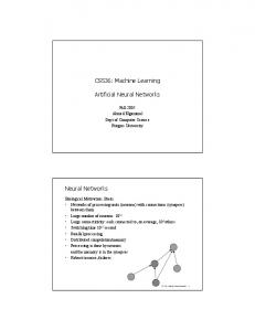
International Journal of Computer Applications (0975 – 8887) Volume 21– No.3, May 2011 IGG covers two shortcomings of the standard SOM approach, namely the necessity to define the size of the map a priori and the problem of cluster boundary detection. To cover these drawbacks, IGG starts with a map of 2*2 neurons. During the training process new neurons are added at the boundary of the map where a large number of input signals are mapped onto a single neuron. Connections between neighboring neurons are added or deleted if the weight vectors assigned to them are ―similar‖ or differ ―a lot‖ in terms of input space distance, thus leading to several sub-networks each consisting of a set of neurons with rather similar weight vectors. These sub-networks represent different clusters of input signals. Thus the map grows in size in order to better represent the input provided. How IGG network topology grows is shown in figure 4. (a) The initial IGG structure after the first organization stage; the boundary neuron with the highest error value is marked. (b) New neurons are grown into any open grid location that is an immediate neighbor of the error neuron. (c) After organizing the new structure with the standard self-organization process, a new error neuron is found. (d) Again, new neurons are grown into any open grid location that is an immediate neighbor of the error neuron. (e) During self-organization of this new structure, the algorithm detects that the circled neurons have developed weight vectors very close in Euclidean distance. (f) These ―close‖ neurons are connected. (g) After further organization, the algorithm discovers connected neighboring neurons whose weight vectors occupy distant areas of the input (i.e., the neurons have a large Euclidean distance). (h) These ―distant‖ neurons are then disconnected in the grid. The incremental grid-growing algorithm is a flexible, dynamic tool for discovering the structure of complicated high-dimensional data. In IGG neurons are added only at the perimeter. The dynamic addition and deletion of connections allows the grid to learn high-dimensional cluster boundaries in the input, avoiding the limitation of standard self-organizing maps. To discover patterns in the data requires both types of knowledge, clustering and topology together in a single representation, but there is no single visualization tool is able to capture both. So analysts must use some combination of these techniques. The Merge clustering only extracts clusters, whereas principal component analysis and the self-organizing map only represent topology. IGG is able to combine both types of information into a single 2-dimensional representation. IGG automatically embeds cluster boundaries into a regular, 2-dimensional topology-preserving network using selforganizing approach using incremental learning. In this manner IGG represents both the cluster boundaries and the highdimensional topology of the input space.
Fig.4. The incremental grid growing network topology Growing new neurons (a)-(d), adding and deleting connection between neighboring neurons (e)-(h)
4.5 Evolve Self-Organizing Maps (ESOM) D. Deng developed the Evolve Self-Organizing Map (ESOM) [16]. The ESOM network starts without neuron that is different from SOM. In ESOM the prototype neurons are not organized onto one or two-dimensional grids and topological constraint is not imposed for the feature map a priori. During learning, the network updates itself with on-line incoming data, creating new neurons when necessary. Each neuron carries a weight vector of the same dimensionality as the input data. Connections between map neurons are used to maintain the neighborhood relationships between close neurons. The strength of the neighborhood relation is determined by the distance between connected neurons. If the distance is too long, the connection can be pruned. In this way the feature map can be split and data structures such as clusters and outliers can emerge. ESOM prototypes are assigned directly using data samples instead of applying an empirical midpoint interpolation. This suggests that whenever data of novelty appear, learning starts with a memory on the data, and continues by adapting the existing memory to the changing environment.
4
International Journal of Computer Applications (0975 – 8887) Volume 21– No.3, May 2011 been applied to the organization of document archives and shows great benefits in the information retrieval area.
4.7 Growing Cell Structures (GCS) The basic building blocks of the generated topology in GCS are hyper-tetrahedrons [18] of a certain dimensionality k chosen in advance. In contrast to SOFM, neither the number of cells nor the exact topology has to be predefined in GCS. Instead, a growth process successively inserts cells and connections. All parameters in the model are constant over time. This makes it possible to continue the growth process until a specific network size is reached or until an application-dependent performance criterion is fulfilled. The input data directly guide the insertion of new cells. Generally, this leads to network structures reflecting the given input distribution better than a predefined topology could. The purpose of the GCS is the generation of a topology-preserving mapping from the input space Rn onto a topological structure A of equal or lower dimensionality k. Topology preservation has such meanings as: (a) Input vectors that are close in Rn should be mapped onto neighboring nodes in A; (b) Neighboring nodes in A should have similar input vectors from Rn mapped onto them.
Fig.5. Neurons insertion and topology of GHSOM The network structure of ESOM is evolved in an on-line adaptive mode. Its features include quick on-line learning ability, a feature map of less geometric constraint, more compactness, and more prototyping accuracy. In ESOM prototypes staying always close to the centre of input data space so it does not suffer from any border effect. Also in ESOM produced neurons are less redundant. It does not have topological folding defects, when part of the map is twisted.
4.6 Growing Hierarchical Maps (GHSOM)
Self-organizing
The GCS generates a k-dimensional topological structure that can be seen as a projection onto a nonlinear, discretely sampled subspace. The GCS starts with a triangle of three cells at random positions in p(x), cells are positioned over the area of non-zero probability density. The insertion of new cells should maintain the triangular connectivity structure. The resulting structure is then redistributed through an adaptive process which is analogous to SOFM, i.e., input vectors are generated according to p(x), then the best matching unit (Vbmu or winner) and its direct topological neighbors (Vdtn) move closer to this vector. The degree by which the winner and its dtn (direct topological neighbor) cells are adapted by constant values, ηwin and ηdtn respectively, here ηwin is greater than ηdtn. The result is a network structure which has reached an equilibrium state where the cell distribution roughly approximates p(x). Figure 5 shows some stages of a simulation for a simple ringshaped data distribution [5].
M. Dittenbach developed the Growing Hierarchical SelfOrganizing Map (GHSOM) [17]. The GHSOM uses a hierarchical architecture. In hierarchical architecture multiple independent layers of SOM is used. Multiple SOM may be used at layers of the hierarchy as shown in figure 5. For every neuron in this map a SOM might be added to the next layer of the hierarchy. This principle is repeated with the third and any further layers of the GHSOM. The size and depth of the hierarchy of the GHSOM is determined during its unsupervised training process. Each layer in the hierarchy consists of a number of independent self-organizing maps which determine their size and arrangement of neurons also during the unsupervised training process. Thus, this model is well suited for applications which require hierarchical clustering of the input data. GHSOM uses a decreasing learning rate and a decreasing neighborhood range instead of fixed values. Of course, the fixed neighborhood range is problematic when the network grows to be larger after a series of insertions. To find out hierarchical relations between input data is a wide spectrum of application domains, thus their proper identification remains a highly important data mining task that cannot be conveniently addressed. But a hierarchical relation between the input data is hard to identify. Due to this problem, GHSOM has
Fig.6. GCS simulation sequence from initial state to final state for a ring-shaped uniform probability distribution Based upon hierarchical clustering and GCS, a Tree-based GCS (Tree GCS) was proposed by V. Hodge [19]. A probabilistic version of the GCS algorithm, Probabilistic GCS (PGCS), was introduced by N. Vlassis [20]. Some new variants and application fields of GCS have been explored. Those examples include: the evolving tree model by J. Pakkanen [21], adaptive self-organizing maps by Y. Yang [22],adaptive topological tree structure by R. Freeman [23].
5
International Journal of Computer Applications (0975 – 8887) Volume 21– No.3, May 2011
5. CONCLUSIONS In GNN using soft competitive learning, there is no need of a priori knowledge of the topology of the network. It can be handled dynamically. Due to the dynamic structure, GNN handles the shortcoming of SOM, which are discussed in second section. In the comparison of fixed topology networks, these growing neural networks have four main characteristics: (1) They can automatically adjust the number of neurons to reflect the complexity of the function that is being interpolated (2) Fast learning ability (3) To obtain the same accuracy; they require fewer weights (4) They can build small networks. The GNN using soft competitive learning can also give a faster speed of convergence because training is done on a growing network, so the weights are less adjusted at each step than in the case of training the fixed topology network at each step.
6. REFERENCES [1] Xinjian Qiang, Guojian Cheng, Zheng Wang An Overview of Some Classical Growing Neural Networks and New Developments, 2nd International Conference on Education Technology and Computer (ICETC), IEEE 2010. [2] Guojian Cheng, Ziqi Song, Jinquan Yang, Rongfang Gao, On Growing Self - Organizing Neural Networks without Fixed Dimensionality, International Conference CIMCAIAWTIC 06 IEEE 2006. [3] B.Fritzke. Growing cell structures- a self-organizing network for unsupervised and supervised learning. Neural Networks, 7(9):1441-1460, 1994. [4] Guojian Cheng, Tianshi Liu, Jiaxin Han, Zheng Wang. Towards Growing Self-Organizing Neural Networks with Fixed networks, Press of Xi' an Jiaotong University, 2008.10, ISBN 978-7-5605-2979-0 (in Chinese). [5] B.Fritzke. Some competitive learning methods. http://www.neuro informatik.ruhr-unibochum.de /ini/ VDM/research/gsn/ JavaPaper/. [6] Self-Organizing Neural Networks without Fixed Dimensionality, Proceedings of CIMCA2006 (International Conference on Computational Intelligence for Modeling, Control and Automation), Published by IEEE Computer Society Press. [7] T. Martinetz, K. Schulten. ‖Neural-Gas‖ network learns topologies. In Proc. International Conference on Artificial Neural Networks (Espoo, Finland), volume I, pages 397– 402, Amsterdam, Netherlands, 1991. [8] T. Martinetz, K. Schulten. Topology representing networks. Neural Networks, 7(2), 1994. [9] T. Martinetz. Competitive Hebbian learning rule forms perfectly topology preserving maps. Int. Conf. on ANN, pages 427–434, London, UK, 1993, Springer.
[12] S. Furao, O. Hasegawa, A Self-organized Growing Network for On-line Unsupervised Learning, IEEE International Joint Conference on Neural Networks (IJCNN2004), CD-ROM ISBN 0-7803-8360-5, Vol.1, pp.11-16 (2004). [13] K. Doherty, R. Adams, N. Davey, TreeGNG -Hierarchical Topological Clustering, Verleysen M.(Eds), In Proceedings of the European Symposium on Artificial Neural Networks (ESANN), 2005. [14] A. Zell, h. Bayer, and h. Bauknecht, Similarity analysis of molecules with self-organizing surfaces—an extension of the self-organizing map. In Proc. icnn’94, International Conference on Neural Networks, pages 719–724, Piscataway, 1994, IEEE Computer Society. [15] J. Blackmore. Visualizing high-dimensional structure with the incremental grid growing neural network. Technical Report AI 95-238, University of Texas, Austin, August 1, 1995. [16] D. Deng and N. Kasabov. ESOM: An algorithm to evolve self-organizing maps from on-line data streams. In Proc. of the International Joint Conference on Neural Networks (IJCNN 2000), volume vi, pages 3 – 8, Como, Italy, July 24. –27. 2000. IEEE Computer Society. [17] M. Dittenbach, D. Merkl and A. Rauber. The growing hierarchical self-organizing map. In Proc. of the International Joint Conference on Neural Networks (IJCNN 2000), volume vi, pages 15 – 19, Como, Italy, July 24. – 27, 2000, IEEE Computer Society. [18] Guojian Cheng, Tianshi Liu, Jiaxin Han, and Zheng Wang, Towards Growing Self-Organizing Neural Networks with Fixed Dimensionality, World Academy of Science, Engineering and Technology 22, 2006. [19] V Hodge, J. Austin. Hierarchical growing cell structures: TreeGCS. In IEEE TKDE Special Issue on Connectionist Models for Learning in Structured Domains. [20] N. Vlassis, A. Dimopoulos, G. Papakonstantinou. The probabilistic growing cell structures algorithm. Lecture Notes in Computer Science, 1327:P649, 1997. [21] J.Pakkanen, J. Iivarinen, E. Oja. The evolving tree - a novel self-organizing network for data analysis. Neural Processing Letters, 20(3):199-211, 2004. [22] Y. Wang, C. Yang, K. Mathee, G. Narasimhan. Clustering using Adaptive Self-Organizing Maps (ASOM) and Applications. Proceedings of International Workshop on Bioinformatics Research and Applications, p944-951 Atlanta, Georgia, May 2005. [23] R. Freeman and H.Yin, "Adaptive Topological Tree Structure (ATSS) for document organization and visualization," Neural Networks, Vol. 17, pp. 1255-1271, 2004.
[10] A.K. Qin, P.N. Suganthan. Robust growing neural gas algorithm with application in cluster analysis, Neural Networks, vol, 17, p.1135-1148, 2004. [11] Y. Prudent, A. Ennaji. A new learning algorithm for incremental self-organizing maps, Verleysen M. (Eds), In Proceedings of the European Symposium on Artificial Neural Networks (ESANN), 2005.
6