that can be used to compute performance measures for a class of QBD processes. .... The solution of the system is derived from first principles using the classic.
Extended abstract submitted for presentation at PMCCS-4
Projection: An efficient solution algorithm for a class of quasi birth-death processes
Gianfranco Ciardo
Evgenia Smirni
Department of Computer Science College of William and Mary Williamsburg, VA 23187-8795 {ciardo,esmirni}@cs.wm.edu
Over the last two decades, considerable effort has been put into the development of matrix geometric techniques [3] for the exact analysis of a general and frequently encountered class of queueing models that exhibit a regular structure. In these models, the embedded Markov chains are two-dimensional generalizations of elementary M/G/1 and G/M/1 queues [1]. The intersection of these two cases corresponds to the so-called quasi-birth-death (QBD) processes. In this work, we develop an efficient methodology that can be used to compute performance measures for a class of QBD processes.
Background: Matrix Geometric Approach If a Markov process exhibits a matrix geometric structure, then its states can be partitioned into two cate(0) (0) (j) (j) gories: the boundary states S (0) = {s1 , . . . , sm } and a sequence of sets of states S (j) = {s1 , . . . , sn }, for j ≥ 1, corresponding to the repetitive portion of the chain. This repetitive structure allows for a recursive formulation of the stationary probabilities of the states in the chain and facilitates their computation. For a QBD process, the infinitesimal generator Q is expressed as [2]: (00) L F(01) 0 0 0 · · · B(10) L(11) F 0 0 · · · B L F 0 ··· (1) Q= 0 , 0 0 B L F ··· .. .. .. .. .. . . . . . . . . where L(00) ∈ IRm×m represents the transition rates between states in S (0) , F(01) ∈ IRm×n represents the transition rates from states in S (0) to states in S (1) , B(10) ∈ IRn×m represents the transition rates from states in S (1) to states in S (0) , F ∈ IRn×n represents transition rates from states in S (j) to states in S (j+1) , L ∈ IRn×n represents transition rates between states in S (j) , B ∈ IRn×n represents transition rates from states in S (j) to states in S (j−1) (for j ≥ 1), and 0 is a matrix of all zeros of the appropriate dimension. Note that we use the mnemonics B (for backward), L (for local), and F (for forward), and that L(11) is usually assumed to equal L (except possibly in the diagonal, since Q is an infinitesimal generator and B(10) · 1T could differ from B · 1T ), but this is not required by our approach (1T is a column vector of ones of the appropriate dimension). Neuts [3] proposed an iterative algorithm that takes advantage of the geometric form of the repetitive
1
portion of the chain to compute the stationary probability vector π of all states, that is, the solution of π · Q = 0. We can partition π as h i π = π (0) , π (1) , π (2) , · · · Let π (j) be the stationary probability vector for states in S (j) (for j ≥ 0). The equation for the repetitive portion of the process in block matrix form is π (j−1) · F + π (j) · L + π (j+1) · B = 0,
j≥2
and since the values of π (j) , j ≥ 2 have a matrix-geometric form, π (j) = π (1) · Gj−1 ,
j ≥ 2,
this implies that the matrix G is the minimal solution of F + G · L + G2 · B = 0. This quadratic equation in the matrix G is typically solved numerically using the following iterative procedure: G(0)
=
0
G(n + 1)
=
−F · L−1 − G2 (n) · B · L−1 ,
n ≥ 0.
To determine the stationary probabilities, one can focus on the equations for the initial portion of the matrix. Observing that π (2) = π (1) · G, this can be written in matrix form as: � h i � L(00) F(01) (0) (1) π ,π · =0 B(10) L(11) + G · B and, together with the normalization condition 1 = π (0) · 1T + π (1) ·
∞ X
Gj−1 · 1T = π (0) · 1T + π (1) · (I − G)−1 · 1T ,
j=1
yields a unique solution. Subsequently, all types of interesting performance metrics (e.g., expected system utilization, throughput, queue length) can be derived.
The Projection Approach We now discuss a class of Markov chains for which a Projection solution is a viable alternative to the classic iterative matrix geometric approach. The advantages of the approach we propose are its simplicity and efficiency. The solution of the system is derived from first principles using the classic Chapman-Kolmogorov [1] equations that relate the flow into and out of each state in equilibrium. Other explicit solution techniques that appear in the literature [4] for the type of chains we consider calculate the stationary probabilities using recursion (i.e., if one knows the stationary probability of state i then the stationary probability of state i + 1 can be determined). The proposed method differs in that we do not evaluate the probability of all states in the chain, rather we compute the aggregate probability distribution for the repetitive portions of the chain. If the repetitive part of the chain is composed of multiple subchains, we compute the aggregate probabilities of each infinite subchain in the system. In 2
S (1) S (0)
s(0) 2
s(0) 1
sm(0)
S (2)
S (3)
s(1) 1
s(2) 1
s(3) 1
R1
s(1) 2
s(2) 2
s(3) 2
R2
s(0) 2
s(0) 3 s(1) n
s(2) n
s(0) 1
(3) s(2) 1 s1
s(1) 2
(3) s(2) 2 s2
s(1) n
(3) s(2) n sn
s(0) 3
Rn
s(3) n
sm(0)
s(1) 1
Figure 1: Partitioning of the state space (left) and its projection (right). (j)
other words our approach explicitly computes the probability of being in each of the n sets R i = {si j ≥ 2}, for 1 ≤ i ≤ n, in steady state (see Fig. 1). More precisely, consider a CTMC exhibiting the QBD structure of Eq. 1. as: (0) (00) π ·L + π (1) ·B(10) = (0) (01) + π (1) ·L(11) + π (2) ·B = π ·F π (1) ·F + π (2) ·L + π (3) ·B = (2) (3) π ·F + π ·L + π (4) ·B = ··· ·
:
Then, we can write π · Q = 0 0 0 0 . 0
(2)
Now, assume that B is a matrix of zeros except for the last column, that is all backward transitions (j) from states in S (j+1) to S (j) are restricted to go to sn , the last state in S (j) . Let A[r1 :r2 ,c1 :c2 ] be the submatrix of A corresponding to the rows from r1 to r2 and the columns from c1 to c2 .
We areP going to show how to derive m + 2n equations in π (0) , π (1) , and a new vector of n unknowns, ∞ (s) π = i=2 π (i) . • The normalization constraint offers one equation:
π (0) · 1T + π (1) · 1T + π (s) · 1T = 1.
(3)
• The first row in (2) provides m equations: π (0) · L(00) + π (1) · B(10) = 0.
(4)
• Due to the structure of B, we can observe that the first n − 1 entries of π (2) · B are null, hence the second row in (2) provides n − 1 equations: (01)
(11)
π (0) · F[1:m,1:n−1] + π (1) · L[1:n,1:n−1] = 0.
(5)
• If we sum all the remaining equations in (2) we obtain ∞ X i=1
π (i) · F +
∞ X
π (i) · L +
i=2
∞ X
π (i) · B = 0,
i=3
which, again by using the structure of B, results in another n − 1 equations: π (1) · F[1:n,1:n−1] + π (s) · (F + L)[1:n,1:n−1] = 0. 3
(6)
• Finally, we can consider the equations describing the balance states, S (j) and S (j+1) , for j = 1, 2, · · ·: (1) T − π (2) ·B·1T = π ·F·1 (2) T π ·F·1 − π (3) ·B·1T = (3) T π ·F·1 − π (4) ·B·1T = ··· ·
of flow between successive sets of 0 0 . 0
By summing all these equations we obtain:
π (1) · F · 1T + π (s) · (F − B) · 1T = 0.
(7)
The above equations are sufficient to compute π (0) , π (1) , and π (s) . Thus, our approach only requires the solution of a linear system in m + 2n variables, and although it does not compute the probability distribution of all individual states, it provides the necessary information to compute the expected stationary value of many Markov reward processes of interest with closed form formulas, such as the expected queue length.
Future Work The condition for the applicability of the Projection approach can be easily described by the structure of matrix B: it must consists of a single nonzero column. However, there are many cases where this condition does not (apparently) hold, but it can still be realized by an appropriate redefinition of the sets S (j) . To decide when this is possible, one only needs to consider the matrices B, L, and F. One example is when B is strictly upper triangular except for a diagonal entry in the last column, and L is upper triangular, but many other combinations are possible. We are in the process of exploring efficient algorithms for automating this repartitioning of the states. An implementation of the Projection approach and a comparison with the Matrix Geometric approach will then be required for timing comparisons.
References [1] L. Kleinrock. Queueing Systems Volume I: Theory. Wiley, 1975. [2] R. Nelson. Matrix geometric solutions in Markov models: a mathematical tutorial. Research Report RC 16777 (#742931), IBM T.J. Watson Res. Center, Yorktown Heights, NY, Apr. 1991. [3] M. Neuts. Matrix-geometric solutions in stochastic models. Johns Hopkins University Press, Baltimore, MD, 1981. [4] P. Snyder and W. Stewart. Explicit and iterative numerical approaches to solving queueing models. Operations Research, 33(1):183–202, Jan-Feb. 1985.
4