Properly embedded minimal planar domains with infinite topology are

arXiv:0909.2326v1 [math.DG] 12 Sep 2009

Properly embedded minimal planar domains with infinite topology are Riemann minimal examples William H. Meeks III∗

Joaqu´ın P´erez †,

September 12, 2009

Abstract These notes outline recent developments in classical minimal surface theory that are essential in classifying the properly embedded minimal planar domains M ⊂ R3 with infinite topology (equivalently, with an infinite number of ends). This final classification result by Meeks, P´erez, and Ros [64] states that such an M must be congruent to a homothetic scaling of one of the classical examples found by Riemann [87] in 1860. These examples Rs , 0 < s < ∞, are defined in terms of the Weierstrass P-functions Pt on the rectangular C elliptic curve h1,t√ , are singly-periodic and intersect each horizontal plane in R3 in a circle −1i or a line parallel to the x-axis. Earlier work by Collin [22], L´opez and Ros [49] and Meeks and Rosenberg [71] demonstrate that the plane, the catenoid and the helicoid are the only properly embedded minimal surfaces of genus zero with finite topology (equivalently, with a finite number of ends). Since the surfaces Rs converge to a catenoid as s → 0 and to a helicoid as s → ∞, then the moduli space M of all properly embedded, non-planar, minimal planar domains in R3 is homeomorphic to the closed unit interval [0, 1]. Mathematics Subject Classification: Primary 53A10, Secondary 49Q05, 53C42.

Contents 1 Introduction.

2

2 Background. 2.1 Weierstrass representation and the definition of flux. . . . . . . . . . . . . . . . . 2.2 Maximum principles. . . . . . . . . . . . . . . . . . . . . . . . . . . . . . . . . . .

5 6 7

∗

This material is based upon work for the NSF under Awards No. DMS - 0405836 and DMS - 0703213. Any opinions, findings, and conclusions or recommendations expressed in this publication are those of the authors and do not necessarily reflect the views of the NSF. † Research partially supported by a MEC/FEDER grant no. MTM2007-61775 and a Junta de Andaluc´ıa grant no. P06-FQM-01642.

1

2.3 2.4 2.5

Monotonicity formula. . . . . . . . . . . . . . . . . . . . . . . . . . . . . . . . . . Stability, Plateau problem and barrier constructions. . . . . . . . . . . . . . . . . The examples that appear in Theorem 1.1. . . . . . . . . . . . . . . . . . . . . .

8 8 10

3 The case with r ends, 2 ≤ r < ∞.

12

4 The one-ended case.

15

5 Infinitely many ends I: one limit end is not possible.

18

6 Infinitely many ends II: two limit ends. 6.1 Curvature estimates and quasiperiodicity. . . . . . . . . . . . . . . . . . . . . . . 6.2 The Shiffman function. . . . . . . . . . . . . . . . . . . . . . . . . . . . . . . . . .

28 29 33

7 Infinitely many ends III: The KdV equation. 7.1 Relationship between the KdV equation and the Shiffman function. . 7.2 Algebro-geometric potentials for the KdV equation. . . . . . . . . . . 7.3 Proof of Theorem 6.11 provided that u is algebro-geometric. . . . . . 7.4 Why u is algebro-geometric if g ∈ Mimm . . . . . . . . . . . . . . . .

45 45 47 48 51

8 The asymptotics of the ends of finite genus surfaces.

1

. . . .

. . . .

. . . .

. . . .

. . . .

. . . .

. . . .

53

Introduction.

In the last decade spectacular progress has been made in various aspects of classical minimal surface theory. Some of the successes obtained are the solutions of open problems which have been pursued since the birth of this subject in the 19-th century, while others have opened vast new horizons for future research. Among the first such successes, we would like to highlight the achievement of a deep understanding of topological aspects of proper minimal embeddings in three-space including their complete topological classification [23, 31, 32, 33, 34, 35, 36]. Equally important in this progress has been a comprehensive analysis of the behavior of limits of sequences of embedded minimal surfaces without a priori area or curvature bounds [9, 15, 16, 17, 18], with outstanding applications such as the classification of all simply-connected, properly embedded minimal surfaces [71]. Also, many deep results have been obtained on the subtle relationship between completeness and properness for complete immersed minimal surfaces [2, 29, 50, 51, 52, 53, 79], and how embeddedness introduces a strong dichotomy in this relationship [21, 61]. While all of these results are extremely interesting, they will not be treated in these notes (at least, not in depth) but they do give an idea of the enormous activity within this field; instead, we will explain the recent solution to the following long standing problem in classical minimal surface theory:

2

Classify all possible properly embedded minimal surfaces of genus zero in R3 . Research by various authors help to understand this problem, the more relevant work being by Colding and Minicozzi [18, 21], Collin [22], L´opez and Ros [49], Meeks, P´erez and Ros [64] and Meeks and Rosenberg [70, 71]. In fact, this problem has been one of main goals of the two authors of these notes (in collaboration with A. Ros) for over the past 15 years, and the long path towards its solution has been marked by the discovery of powerful techniques which have proved useful in other applications. Putting together all of these efforts, we now state the final solution to the above problem, whose proof appears in [64]. Theorem 1.1 Up to scaling and rigid motion, any connected, properly embedded, minimal planar domain in R3 is a plane, a helicoid, a catenoid or one of the Riemann minimal examples1 . In particular, for every such surface there exists a foliation of R3 by parallel planes, where each plane intersects the surface transversely in a circle or a straight line. In these notes we will try to pass on to the reader a glimpse of the beauty of the arguments and different theories that intervene in the proof of Theorem 1.1. Among these auxiliary theories, we highlight the theory of integrable systems, whose applications to minimal and constant mean curvature surface theory have gone far beyond the existence results in the late eighties (Abresch [1], Bobenko [5], Pinkall and Sterling [85], based on the sinh-Gordon equation) to recent uniqueness theorems like the one that gives the title of these notes (based on the KdV equation), and the even more recent tentative solution to the Lawson conjecture by Kilian and Schmidt [45]. Before proceeding, we make a few general comments about the organization of this article, which relate to the proof of Theorem 1.1. In Section 2 we briefly introduce the main definitions and background material, including short discussions of the classical examples that appear in the statement of the above theorem. Since a complete, immersed minimal surface M without boundary in R3 cannot be compact, M must have ends2 . As we are interested in planar domains, the allowed topology for our surfaces in that of the two-sphere minus a compact totally disconnected set E 6= Ø corresponding to the space of ends of the surface. A crucial result proved by Collin [22] in 1997 (see Conjecture 3.3 below) implies that when the cardinality #(E) of E satisfies 2 ≤ #(E) < ∞, then the total Gaussian curvature of M is finite. Complete embedded minimal surfaces with finite total curvature comprise the best understood minimal surfaces in R3 ; the main reason for this is the fact discovered by Osserman that the underlying complex structure for every such minimal surface M is that of a compact Riemann M surface minus a finite number of points, and the classical analytic Weierstrass representation data on M extends 1

See Section 2.5 for further discussion of these surfaces. An end of a non-compact connected topological manifold M is an equivalence class in the set A = {α : [0, ∞) → M | α is a proper arc}, under the equivalence relation: α1 ∼ α2 if for every compact set C ⊂ M , α1 , α2 lie eventually in the same component of M − C. If α ∈ A is a representative proper arc of and end of M and Ω ⊂ M is a proper subdomain with compact boundary such that α ⊂ Ω, then we say that Ω represents the end e. 2

3

across the punctures to meromorphic data on M . Using the maximum principle together with their result that every complete, embedded minimal surface with genus zero and finite total curvature can be minimally deformed, L´opez and Ros characterized the plane and the catenoid as being the unique embedded examples of finite total curvature and genus zero, see Theorem 3.2. We also explain Collin’s and L´ opez-Ros’ theorems in Section 3. Section 4 covers the one-ended case of Theorem 1.1, which was solved by Meeks and Rosenberg (Theorem 4.2). To understand the proof of this result we need the local results of Colding and Minicozzi which describe the structure of compact, embedded minimal disks as essentially being modeled by either a plane or a helicoid, and their one-sided curvature estimate together with other results of a global nature such as their limit lamination theorem for disks, see Theorem 4.1 below. The remainder of the article, except for the last section, focuses on the case in Theorem 1.1 where the surface has infinitely many ends. Crucial in this discussion is the Ordering Theorem by Frohman and Meeks (Theorem 5.1) as well as two topological results, the first on the nonexistence of middle limit ends due to Collin, Kusner, Meeks and Rosenberg (Theorem 5.3) and the second on the non-existence of properly embedded minimal planar domains with just one limit end by Meeks, P´erez and Ros (Theorem 5.11). It follows from these two non-existence results that a properly embedded minimal planar domain must have exactly two limit ends. These key ingredients represent the content of Section 5. As a consequence of the results in Section 5, in Section 6 we obtain strong control on the conformal structure and height differential of a properly embedded, minimal planar domain M with infinitely many ends. In this section we also explain how Colding-Minicozzi theory can be applied to obtain a curvature bound for such an M , after it has been the normalized by a homothety so that its vertical flux is 1, which only depends on the length of the horizontal component of its flux vector (Theorem 6.3). This bound leads to a quasi-periodicity property of M , which is a cornerstone to finishing the classification problem. Also in Section 6 we introduce the Shiffman Jacobi function SM and explain how the existence of a related holomorphic deformation of M preserving its flux is sufficient to reduce the proof of Theorem 1.1 in the case with infinitely many ends to the singly-periodic case, which was solved earlier by Meeks, P´erez and Ros [66]. In Section 7 we explain how the existence of the desired holomorphic deformation of M follows from the integration of an evolution equation for its Gauss map. The Shiffman function SM will be crucial at this point by enabling us to reduce this evolution equation to an equation of type Korteweg de Vries (KdV). A classical condition that implies global integrability of the KdV equation, i.e. existence of (globally defined) meromorphic solutions u(z, t) of the Cauchy problem associated to the KdV equation, is that the initial condition u(z) is an algebro-geometric meromorphic function, a concept related to the hierarchy of the KdV equation. In our setting, the final step of the classification of the properly embedded minimal planar domains consists of proving that the initial condition u(z) for the Cauchy problem of the KdV equation naturally associated to any quasiperiodic, possibly immersed, minimal planar domain M with two limit 4

ends is algebro-geometric (Section 7.4), which in turn is a consequence of the fact that the space of bounded Jacobi functions on such a surface M is finite dimensional (Theorem 7.3). An important consequence of the proof of the classification of properly embedded minimal planar domains is the characterization of the asymptotic behavior of the ends of any properly embedded minimal surface M ⊂ R3 with finite genus. If e ∈ E(M ) is an end, then there exists properly embedded domain E(e) ⊂ M with compact boundary which represents e and such that in a natural sense E(e) converges to the end of a plane, a catenoid, a helicoid or to one of the limit ends of a Riemann minimal example. This asymptotic characterization is due to Schoen [91] and Collin [22] when M has a finite number of ends greater than one, to Meeks, P´erez and Ros in the case M has an infinite number of ends, and to Meeks and Rosenberg [71], Bernstein and Breiner [3], and Meeks and P´erez [58, 59] in the case of just one end. These asymptotic characterization results will be explained in Section 8 of these notes.

2

Background.

An isometric immersion X = (x1 , x2 , x3 ) : M → R3 of a Riemannian surface into Euclidean space is said to be minimal if xi is a harmonic function on M for each i (in the sequel, we will identify the Riemannian surface M with its image under the isometric embedding). Since harmonicity is a local property, we can extend the notion of minimality to immersed surfaces M ⊂ R3 . We will always assume all surfaces under consideration are orientable. If M ⊂ R3 is an immersed oriented surface, we will denote by H the mean curvature function of X (average normal curvature) and by N : M → S2 (1) ⊂ R3 its Gauss map. Since ∆X = 2HN (here ∆ is the Laplace-Beltrami operator on M ), we have that M is minimal if and only if H = 0 identically. Expressing locally M as the graph of a function u = u(x, y) (after a rotation), the last equation can be written as the following quasilinear second order elliptic PDE: ! ∇0 u div0 p = 0, (1) 1 + |∇0 u|2 where the subscript •0 indicates that the corresponding object is computed with respect to the flat metric in the plane. Let Ω be a subdomain with compact closure in a surface M ⊂ R3 and let u ∈ C0∞ (Ω) be a compactly supported smooth function. The first variation of the area functional A(t) = Area((X +tuN )(Ω)) for the normally perturbed immersions X +utN (with |t| sufficiently small) gives Z A0 (0) = −2

uH dA,

(2)

Ω

where dA stands for the area element of M . Therefore, M is minimal if and only if it is a critical point of the area functional for all compactly supported variations. The second variation of area implies that any point in a minimal surface has a neighborhood with least-area relative to its 5

boundary3 , and thus M ⊂ R3 is minimal if and only if every point p ∈ M has a neighborhood with least-area R relative to its boundary. If one exchanges the area functional A by the Dirichlet energy E = Ω |∇X|2 dA, then the two functionals are related by E ≥ 2A, with equality if and only if the immersion X : M → R3 is conformal. This relation between area and energy together with the existence of isothermal coordinates on every Riemannian surface allow us to state that a conformal immersion X : M → R3 is minimal if and only if it is a critical point of the Dirichlet energy for all compactly supported variations (or equivalently, every point p ∈ M has a neighborhood with least energy relative to its boundary). Finally, the relation Ap = −dNp between the differential of the Gauss map and the shape operator, together with the CauchyRiemann equations give that M is minimal if and only if its stereographically projected Gauss map g : M → C ∪ {∞} is a holomorphic function. All these equivalent definitions of minimality illustrate the wide variety of branches of mathematics that appear in its study: Differential Geometry, PDE, Calculus of Variations, Geometric Measure Theory, Complex Analysis, etc. The Gaussian curvature function4 K of a surface M ⊂ R3 can be written as K = κ1 κ2 = det A, where κi are the principal curvatures and A the shape operator. Thus |K| is the absolute value of the Jacobian of the Gauss map N . If M is minimal, then κ1 = −κ2 and K ≤ 0, hence the total curvature C(M ) of M is the negative of the spherical area of M through its Gauss map, counting multiplicities: Z C(M ) = K dA = −Area(N : M → S2 (1)) ∈ [−∞, 0]. (3) M

In the sequel, we will denote by B(p, R) = {x ∈ R3 | |x − p| < R} and B(R) = B(~0, R).

2.1

Weierstrass representation and the definition of flux.

Let M ⊂ R3 be a possibly immersed minimal surface, with stereographically projected Gauss map g : M → C ∪ {∞}. Since the third coordinate function x3 of M is harmonic, it admits a locally well-defined harmonic conjugate function x∗3 . The height differential of M is the holomorphic 1-form dh = dx3 + idx∗3 (note that dh is not necessarily exact on M ). The minimal immersion X : M → R3 can be written up to translation by the vector X(p0 ), p0 ∈ M , solely in terms of the Weierstrass data (g, dh) as     Z p  1 1 i 1 X(p) = < −g , + g , 1 dh, (4) 2 g 2 g p0 where < stands for real part. The positive-definiteness of the induced metric and the independence of (4) with respect to the integration path give rise to certain compatibility conditions 3

This property justifies the word “minimal” for these surfaces. If needed, we will use the notation KM to highlight the surface M of which K is the Gaussian curvature function. 4

6

on the meromorphic data (g, dh) for analytically defining a minimal surface (Osserman [80]); namely, if we start with a meromorphic function g and a holomorphic one-form dh on an abstract Riemann surface M , then the map X : M → R3 given by (4) is a conformal minimal immersion with Weierstrass data (g, dh) provided that two conditions hold: The zeros of dh coincide with the poles and zeros of g, with the same order. Z

Z g dh = γ

γ

dh , g

(5)

Z dh = 0 for any closed curve γ ⊂ M (period problem).


0} by Theorem 2.1) but is not contained in {x3 > c} for any c > 0. Since M is proper, we can find a ball B(p, r) centered at a point p ∈ {x3 = 0} such that M ∩ B(p, r) = Ø. Consider a vertical half-catenoid C with negative 7

logarithmic growth, completely contained in {x3 ≤ 0} ∪ B(p, r), whose waist circle Γ is centered at q = p + ε(0, 0, 1), ε > 0 small. Then M ∩ C = Ø. Now deform C = C(1) by a one-parameter family of non-compact annular pieces of vertical catenoids {C(r)}r∈(0,1] , all having the same boundary Γ as C, with negative logarithmic growths converging to zero as r → 0 and whose Gaussian curvatures blow up at a the limit point of the waist circles of C(r), which is the point q. Then, the surfaces C(r) converge on compact subsets of R3 − {q} to the plane {x3 = ε}, and so, M achieves a first contact point with one of the catenoids, say C(r0 ), in this family; the usual maximum principle for M and C(r0 ) gives a contradiction. 2 Theorem 2.3 (Maximum Principle at Infinity [73]) Let M1 , M2 ⊂ R3 be disjoint, connected, properly immersed minimal surfaces with (possibly empty) boundary. i) If ∂M1 6= Ø or ∂M2 6= Ø, then after possibly re-indexing, dist(M1 , M2 ) = inf{dist(p, q) | p ∈ ∂M1 , q ∈ M2 }. ii) If ∂M1 = ∂M2 = Ø, then M1 and M2 are flat.

2.3

Monotonicity formula.

Monotonicity formulas, as well as maximum principles, play a crucial role in many areas of Geometric Analysis. For instance, we will see in Theorem 5.3 how the monotonicity formula can be used to discard middle limit ends for a properly embedded minimal surface. We will state this basic result without proof here; it is a consequence of the classical coarea formula applied to the distance function to a point p ∈ R3 , see for instance Corollary 4.2 in [14] for a detailed proof. Theorem 2.4 (Monotonicity Formula [10, 46]) Let X : M → R3 be a connected, properly immersed minimal surface. Given p ∈ R3 , let A(R) = Area(X(M ) ∩ B(p, R)). Then, A(R)R−2 is non-decreasing. In particular, limR→∞ A(R)R−2 ≥ π with equality if and only if M is a plane.

2.4

Stability, Plateau problem and barrier constructions.

Recall that every (orientable) minimal surface M ⊂ R3 is a critical point of the area functional for compactly supported normal variations. M is said to be stable if it is a local minimum for such a variational problem. The following well-known result indicates how restrictive is stability for complete minimal surfaces. It was proved independently by Fischer-Colbrie and Schoen [30], do Carmo and Peng [25], and Pogorelov [86] for orientable surfaces and more recently by Ros [89] in the case of non-orientable surfaces. Theorem 2.5 If M ⊂ R3 is a complete, immersed, stable minimal surface, then M is a plane. 8

The Plateau Problem consists of finding a compact surface of least area spanning a given boundary. This problem can be solved under certain circumstances; this existence of compact solutions together with a taking limits procedure leads to construct non-compact stable minimal surfaces in R3 that are constrained to lie in regions of space whose boundaries have non-negative mean curvature. A huge amount of literature is devoted to this procedure, but we will state here only a particular version. Let W be a compact Riemannian three-manifold with boundary which embeds in the interior of another Riemannian three-manifold. W is said to have piecewise smooth, mean convex boundary if ∂W is a two-dimensional complex consisting of a finite number of smooth, two-dimensional compact simplices with interior angles less than or equal to π, each one with non-negative mean curvature with respect to the inward pointing normal. In this situation, the boundary of W is a good barrier for solving Plateau problems in the following sense: Theorem 2.6 ([54, 75, 76, 94]) Let W be a compact Riemannian three-manifold with piecewise smooth mean convex boundary. Let Γ be a smooth collection of pairwise disjoint closed curves in ∂W , which bounds a compact orientable surface in W . Then, there exists an embedded orientable surface Σ ⊂ W with ∂Σ = Γ that minimizes area among all orientable surfaces with the same boundary. Instead of giving an idea of the proof of Theorem 2.6, we will illustrate it together with a taking limits procedure to obtain a particular result in the non-compact setting. Consider two disjoint, connected, properly embedded minimal surfaces M1 , M2 in R3 and let W be the closed complement of M1 ∪ M2 in R3 that has both M1 and M2 on its boundary. 1. We first show how to produce compact, least-area surfaces in W with prescribed boundary lying in the boundary ∂W . Note that W is a complete flat three-manifold with boundary, and ∂W has mean curvature zero. Meeks and Yau [76] proved that W embeds isometrically f diffeomorphic to the interior in a homogeneously regular5 Riemannian three-manifold W of W and with metric ge. Morrey [78] proved that in a homogeneously regular manifold, one can solve the classical Plateau problem. In particular, if Γ is an embedded 1-cycle f which bounds an orientable finite sum of differentiable simplices in W f , then by in W standard results in geometric measure theory [28], Γ is the boundary of a compact, leastf . Meeks and Yau proved that the metric ge on W f can area embedded surface ΣΓ (e g) ⊂ W f , which be approximated by a family of homogeneously regular metrics {gn }n∈N on W f converges smoothly on compact subsets of W to ge, and each gn satisfies a convexity f , which forces the least-area surface ΣΓ (gn ) to lie in W if condition outside of W ⊂ W Γ lies in W . A subsequence of the ΣΓ (gn ) converges to a smooth minimal surface ΣΓ of 5

A Riemannian three-manifold N is homogeneously regular if given ε > 0 there exists δ > 0 such that δ-balls in N are ε-uniformly close to δ-balls in R3 in the C 2 -norm. In particular, if N is compact, then N is homogeneously regular.

9

least-area in W with respect to the original flat metric, thereby finishing our description of how to solve (compact) Plateau-type problems in W . 2. We now describe the limit procedure to construct a non-compact, stable minimal surface with prescribed boundary lying in M1 . Let M1 (1) ⊂ . . . ⊂ M1 (n) ⊂ . . . be a compact exhaustion of M1 , and let Σ1 (n) be a least-area surface in W with boundary ∂M1 (n), constructed as in the last paragraph. Let α be a compact arc in W which joins a point in M1 (1) to a point in ∂W ∩ M2 . By elementary intersection theory, α intersects every least-area surface Σ1 (n). By compactness of least-area surfaces, a subsequence of the surfaces Σ1 (n) converges to a properly embedded area-minimizing surface Σ in W with a component Σ0 which intersects α; this proof of the existence of Σ is due to Meeks, Simon and Yau [74]. 3. We finish this application of the barrier construction, as follows. Since Σ0 separates R3 , Σ0 is orientable and so, Theorem 2.5 insures that Σ0 is a plane. Hence, M1 and M2 lie in closed half-spaces of R3 , and the Half-space Theorem (Theorem 2.2) implies that both M1 , M2 are planes. The above items 1–3 give the following generalization of Theorem 2.2, also due to Hoffman and Meeks. Theorem 2.7 (Strong Half-space Theorem [41]) If M1 and M2 are two disjoint, properly immersed minimal surfaces in R3 , then M1 and M2 are parallel planes.

2.5

The examples that appear in Theorem 1.1.

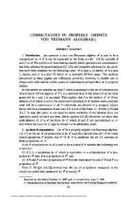
We will now use the Weierstrass representation for introducing the minimal planar domains characterized in Theorem 1.1. The plane. M = C, g(z) = 1, dh = dz. It is the only complete, flat minimal surface in R3 . The catenoid. M = C − {0}, g(z) = z, dh = dz z (Figure 1 left). This surface has genus zero, two ends and total curvature −4π. Together with the plane, the catenoid is the only minimal surface of revolution (Bonnet [6]). As we will see in Theorem 3.2, the catenoid and the plane are the unique complete, embedded minimal surfaces with genus zero and finite total curvature. Also, the catenoid was characterized by Schoen [91] as being the unique complete, immersed minimal surface with finite total curvature and two embedded ends. The helicoid. M = C, g(z) = ez , dh = i dz (Figure 1 center). When viewed in R3 , the helicoid has genus zero, one end and infinite total curvature. Together with the plane, the helicoid is the only ruled minimal surface (Catalan [8]), and we will see in Theorem 4.2 below that it is the unique properly embedded, simply-connected minimal surface. The vertical helicoid is invariant

10

Figure 1: Left: Catenoid. Center: Helicoid. Right: One of the Riemann minimal examples. Figures courtesy of Matthias Weber.

by a vertical translation T and by a 1-parameter family of screw motions6 Sθ , θ > 0. Viewed in R3 /T or in R3 /Sθ , the helicoid is a properly embedded minimal surface with genus zero, two ends and finite total curvature. The catenoid and the helicoid are conjugate minimal surfaces, in the sense that the coordinate functions of one of these surfaces are the harmonic conjugates of the coordinate functions of the other one; in this case, we consider the catenoid to be defined on its universal cover ez : C → C − {0} in order for the harmonic conjugate of x3 to be well-defined. The Riemann minimal examples. They form a one-parameter family, with Weierstrass data Mλ = {(z, w) ∈ (C ∪ {∞})2 | w2 = z(z − λ)(λz + 1)} − {(0, 0), (∞, ∞)}, g(z, w) = z, dh = Aλ dz w, 2 for each l > 0, where Aλ is a non-zero complex number satisfying Aλ ∈ R (one of these surfaces is represented in Figure 1 right). Together with the plane, catenoid and helicoid, these examples were characterized by Riemann [88] as the unique minimal surfaces which are foliated by circles and lines in parallel planes. Each Riemann minimal example Ml is topologically a cylinder minus an infinite set of points which accumulates at infinity to the top or bottom ends of the cylinder; hence, Ml is topologically the unique planar domain with two limit ends. Furthermore, Ml is invariant under reflection in the (x1 , x3 )-plane and by a translation Tl ; the quotient surface Ml /Tl ⊂ R3 /Tl has genus one and two planar ends, provided that Tl is the generator of the orientation preserving translations of Mλ . The conjugate minimal surface of Ml is M1/l (the case l = 1 gives the only self-conjugate surface in the family). See [64] for a more precise description of these surfaces. 6

A screw motion Sθ is the composition of a rotation of angle θ around the x3 -axis with a translation in the direction of this axis.

11

3

The case with r ends, 2 ≤ r < ∞.

Complete minimal surfaces with finite total curvature can be naturally thought of as compact algebraic objects, which explains why these surfaces form the most extensively studied family among complete minimal surfaces. Theorem 3.1 (Huber [42], Osserman [81]) Let M ⊂ R3 be a complete (oriented), immersed minimal surface with finite total curvature. Then, M is conformally a compact Riemann surface M minus a finite number of points, and the Weierstrass representation (g, dh) of M extends meromorphically to M . In particular, the total curvature of M is a multiple of −4π. Under the hypotheses of the last theorem, the Gauss map g has a well-defined finite degree on M , and equation (3) implies that the total curvature of M is −4π times the degree of g. The Gauss-Bonnet formula relates the degree of g with the genus of M and the number of ends (Jorge and Meeks [43]); although this formula can be stated in the more general immersed case, we will only consider it when all the ends of M are embedded: deg(g) = genus(M ) + #(ends) − 1.

(8)

The asymptotics of a complete, embedded minimal surface in R3 with finite total curvature are also well-understood: after a rotation, each embedded end of such a surface is a graph over the exterior of a disk in the (x1 , x2 )-plane with height function x3 (x1 , x2 ) = a log r + b +

c1 x1 + c2 x2 + O(r−2 ), r2

(9)

p where r = x21 + x22 , a, b, c1 , c2 ∈ R and O(r−2 ) denotes a function such that r2 O(r−2 ) is bounded as r → ∞ (Schoen [91]). When the logarithmic growth a in (9) is not zero, the end is called a catenoidal end (and the surface is asymptotic to a half-catenoid); if a = 0, we have a planar end (and the surface is asymptotic to a plane). A consequence of the asymptotics (9) is that for minimal surfaces with finite total curvature, completeness is equivalent to properness (this is also true for immersed surfaces). The classification of the complete embedded minimal surfaces with genus zero and finite total curvature in R3 was solved in 1991 by L´opez and Ros [49]. Their result is based on the fact that every surface in this family can be deformed through minimal surfaces of the same type; this is a strong property which we will encounter in more general situations, as in Theorem 6.11 below. In the finite total curvature setting, the deformation is explicitly given in terms of the Weierstrass representation: If (g, dh) is the Weierstrass pair of a minimal surface M , then for each l > 0 the pair (lg, dh) satisfies condition (5) and the second equation in (6). The first equation in (6) holds for (lg, dh) provided that the flux vector F (γ) of M along every closed curve γ ⊂ M is vertical. If M is assumed to have genus zero and finite total curvature, then 12

the homology classes of M are generated by loops around its planar and/or catenoidal ends. It is easy to check that the flux vector of a catenoidal (resp. planar) end along a non-trivial loop is (0, 0, ±2πa) after assuming that the limiting normal vector at the end is (0, 0, ±1). Since embeddedness implies that all the ends are parallel, then all the flux vectors of our complete embedded minimal surface M with genus zero and finite total curvature are vertical; hence (lg, dh) defines a minimal immersion Xl by the formula (4) for each l > 0; note that for l = 1 we obtain the starting surface M . A direct consequence of the maximum principle is that smooth deformations of compact minimal surfaces remain embedded away from their boundaries. The strong control on the asymptotics for complete embedded minimal surfaces of finite total curvature implies embeddedness throughout the entire deformation {Xl }l>0 . This last property excludes both points in M with horizontal tangent plane and planar ends (a local analysis of the deformation around such points and ends produce self-intersections in Xl for values of the parameter l close to zero or infinity), which in turn implies that the height function x3 of M is proper without critical points. A simple application of Morse theory gives that M has just two ends, in which case the characterization of the catenoid was previously solved by Schoen [91]. This is a sketch of the proof of the following result. Theorem 3.2 (L´ opez, Ros [49]) The plane and the catenoid are the only complete, embedded minimal surfaces in R3 with genus zero and finite total curvature. The next step in our classification of all properly embedded minimal planar domains is to understand the case when the number of ends is finite and at least two. In 1993, Meeks and Rosenberg [70] showed that if a properly embedded minimal surface M ⊂ R3 has at least two ends, then every annular end E ⊂ M either has finite total curvature or it satisfies the hypotheses of the following conjecture, which was solved by Collin in 1997. Conjecture 3.3 (Generalized Nitsche Conjecture, Collin’s Theorem [22]) Let E ⊂ {x3 ≥ 0} be a properly embedded minimal annulus with ∂E ⊂ {x3 = 0}, such that E intersects each plane {x3 = t}, t > 0, in a simple closed curve. Then, E has finite total curvature. As a direct consequence of the last result and Theorem 3.2, we have that the plane and the catenoid are the unique properly embedded minimal surfaces in R3 with genus zero and r ends, 2 ≤ r < ∞. Collin’s original proof of Conjecture 3.3 is a beautiful and long argument based on the construction of auxiliary minimal graphs which serve as guide posts to elucidate the shape of E in space. For later purposes, it will be more useful for us to briefly explain a later proof due to Colding and Minicozzi, which is based on the following scale invariant bound for the Gaussian curvature of any embedded minimal disk in a half-space.

13

Theorem 3.4 (One-sided curvature estimates, Colding, Minicozzi [18]) There exists ε > 0 such that the following holds. Given r > 0 and an embedded minimal disk M ⊂ B(2r) ∩ {x3 > 0} with ∂M ⊂ ∂B(2r), then for any component M 0 of M ∩ B(r) which intersects B(εr), sup |KM | ≤ r−2 . M0

Before sketching the proof of the Nitsche Conjecture, we will make a few comments about the one-side curvature estimates. The catenoid shows that the hypothesis in Theorem 3.4 on M to be simply-connected is necessary. Theorem 3.4 implies that if an embedded minimal disk is close enough to (and lies at one side of) a plane, then reasonably large components of it are graphs over this plane. The proof of Theorem 3.4 is long and delicate, see [15, 16, 18]. Returning to the Nitsche Conjecture, we see that itpfollows directly from the next result. Given ε ∈ R, we denote by Cε the conical region {x3 > ε x21 + x22 }. Theorem 3.5 (Colding, Minicozzi [11]) There exists δ > 0 such that any properly embedded minimal annular end E ⊂ C−δ has finite total curvature. Sketch of proof of Theorem 3.5. The argument starts by showing, for each δ > 0, the existence of a sequence {yj }j ⊂ E −Cδ with kyj k → ∞ (this is done by contradiction: if for a given δ > 0 this property fails, then one use E together with the boundary of Cδ as barriers to construct an end of finite total curvature contained in Cδ , which is clearly impossible by the controlled asymptotics of catenoidal and planar ends). The next step consists of choosing suitable radii rj > 0 such that the connected component Mj of E ∩ B(yj , 2rj ) which contains yj is a disk. Now if δ > 0 is sufficiently small in terms of the ε appearing in the one-sided curvature estimates, we can apply Theorem 3.4 and conclude a bound for the supremum of the absolute Gaussian curvature of the component Mj1 of Mj ∩ B(yj , rj ) which contains yj . A Harnack type inequality together with this curvature bound gives a bound for the length of the intrinsic gradient of x3 in the intrinsic ball Bj in Mj1 centered at yj with radius 5rj /8, which in turn implies (by choosing ε sufficiently small) that Bj is a graph with small gradient over x3 = 0, and one can control a bound by below of the diameter of this graph. This allows to repeat the above argument exchanging yj by a point yj1 in Bj1 at certain distance from yj , and the estimates are carefully done so that the procedure can be iterated to go entirely around a curve γj ⊂ E whose projection to the (x1 , x2 )-plane links once around the x3 -axis. The graphical property of γj implies that either γj can be continued inside E to spiral indefinitely or it closes up with linking number one with the x3 -axis. The first possibility contradicts that E is properly embedded, and in the second case the topology of E implies that ∂E ∪ γj bounds an annulus Ej . The above gradient estimate gives a linear growth estimate for the length of γj in terms of kyj k, from where the isoperimetric inequality for doubly connected minimal surfaces by Osserman and Schiffer [82] gives a quadratic growth estimate for the area of Ej . Finally, this quadratic area growth property together with the finiteness of the topology of E imply that E has finite total curvature by the Gauss-Bonnet formula, finishing the outline of proof. 14

4

The one-ended case.

In our goal of classifying the properly embedded minimal surfaces with genus zero, the simplest topology occurs when the number of ends is one, and the surface is simply-connected. In spite of this apparent simplicity, this problem remained open until 2005, when Meeks and Rosenberg gave a complete solution by using the one-side curvature estimates (Theorem 3.4) and other aspects of Colding-Minicozzi theory that we comment on in this section. Classical minimal surface theory allows us to understand the structure of limits of sequences of embedded minimal surfaces with fixed genus, when the sequence has uniform local area and curvature bounds, see for instance the survey by P´erez and Ros [84]. Colding and Minicozzi faced the same problem in the absence of such uniform local bounds in a series of papers starting in 2004 [9, 15, 16, 17, 18]. Their most important structure theorem deals with the case in which all minimal surfaces in the sequence are disks whose Gaussian curvature blows up near the origin. To understand this phenomenon, one should think of a sequence of rescaled helicoids Mn = ln H = {ln x | x ∈ H}, where H is a fixed vertical helicoid with axis the x3 -axis and ln ∈ R+ , ln & 0. The curvature of the sequence {Mn }n blows up along the x3 -axis and the Mn converge away from the axis to the foliation L of R3 by horizontal planes. The x3 -axis is the singular set of C 1 -convergence S(L) of Mn to L, and each leaf L of L extends smoothly across L ∩ S(L) (i.e. S(L) consists of removable singularities of L). The same behavior is mimicked by any sequence of embedded minimal disks in balls centered at the origin with radii tending to infinity: Theorem 4.1 (Limit Lamination Theorem for Disks, Colding, Minicozzi [18]) Let Mn ⊂ B(Rn ) be a sequence of embedded minimal disks with ∂Mn ⊂ ∂B(Rn ) and Rn → ∞. If sup |KMn ∩B(1) | → ∞, then there exists a subsequence of the Mn (denoted in the same way) and a Lipschitz curve S : R → R3 such that up to a rotation of R3 , 1. x3 (S(t)) = t for all t ∈ R. 2. Each Mn consists of exactly two multigraphs7 away from S(R) which spiral together. 3. For each α ∈ (0, 1), the surfaces Mn − S(R) converge in the C α -topology to the foliation L = {x3 = t}t∈R by horizontal planes. 4. sup |KMn ∩B(S(t),r) | → ∞ as n → ∞, for any t ∈ R and r > 0. Sketch of proof. Similar as in the proof of the one-sided curvature estimates (Theorem 3.4), the proof of this theorem is involved and runs through various papers [15, 16, 18] (references [13, 12, 14, 19, 20] by Colding and Minicozzi are reading guides for the complete proofs of these results). We will content ourselves with a rough idea of the argument. The first step consists of showing that the embedded minimal disk Mn with large curvature at some interior point can be

15

divided into multivalued graphical building blocks un (ρ, θ) defined on annuli7 , and that these basic pieces fit together properly, in the sense that the number of sheets of un (ρ, θ) rapidly grows as the curvature blows up and at the same time, the sheets do not accumulate in a half-space. This is obtained by means of sublinear and logarithmic bounds for the separation7 wn (ρ, θ) as a function of ρ → ∞. Another consequence of these bounds is that by allowing the inner radius7 of the annulus where the multigraph is defined to go to zero, the sheets of this multigraph collapse (i.e. |wn (ρ, θ)| → 0 as n → ∞ for ρ, θ fixed); thus a subsequence of the un converges to a smooth minimal graph through ρ = 0. The fact that the Rn go to ∞ then implies this limit graph is entire and, by the classical Bernstein’s Theorem [4], it is a plane. The second step in the proof uses the one-sided curvature estimates in the following manner: once it has been proven that an embedded minimal disk M contains a highly sheeted double f, then M f plays the role of the plane in the one-sided curvature estimate, which multigraph M implies that reasonably large pieces of M consist of multigraphs away from a cone with axis “orthogonal” to the double multigraph. The fact that the singular set of convergence is a Lipschitz curve follows because the aperture of this cone is universal (another consequence of Theorem 3.4). 2 With the above discussion in mind, we can now state the main result of this section. Theorem 4.2 (Meeks, Rosenberg [71]) If M ⊂ R3 is a properly embedded, simply-connected minimal surface, then M is a plane or a helicoid. Sketch of Proof. Take a sequence {λn }n ⊂ R+ with ln → 0 as n → ∞, and consider the rescaled surface λn M . Since M is simply-connected, Theorem 4.1 gives that a subsequence of ln M converges on compact subsets of R3 to a minimal foliation L of R3 by parallel planes, with singular set of convergence S(L) being a Lipschitz curve that can be parameterized by the height over the planes in L. Furthermore, a consequence of the proof of Theorem 4.1 in our case is that for n large, the almost flat multigraph which starts to form on ln M near the origin extends all the way to infinity. From here in can be shown that the limit foliation L is independent of the sequence {λn }n . After a rotation of M and replacement of the ln M by a subsequence, we can suppose that the ln M converge to the foliation L of R3 by horizontal planes, on compact subsets outside of the singular set of convergence given by a Lipschitz curve S(L) parameterized by its x3 -coordinate. In particular, S(L) intersects each horizontal plane exactly once. The next step consists of proving that M intersects transversely each of the planes in L. The idea now is to consider the solid vertical cylinder E = {x21 + x22 ≤ 1, −1 ≤ x3 ≤ 1}. After a homothety and translation, we can assume that S(L)∩{x3 = 0} = {~0} and S(L)∩{−1 ≤ x3 ≤ 1} is contained in the convex component of the solid cone whose boundary has the origin as vertex and that passes through the circles in ∂E. The Colding-Minicozzi picture of Theorem 4.1 7

In polar coordinates (ρ, θ) with ρ > 0 and θ ∈ R, a k-valued graph on an annulus of inner radius r and outer radius R, is a single-valued graph of a function u(ρ, θ) defined over {(ρ, θ) | r ≤ ρ ≤ R, |θ| ≤ kπ}, k being a positive integer. The separation between consecutive sheets is w(ρ, θ) = u(ρ, θ + 2π) − u(ρ, θ) ∈ R.

16

implies that for n large, ln M intersects ∂E ∩ {−1 < x3 < 1} in a finite number of spiraling curves. For simplicity, we will suppose additionally that the foliation of ∂E ∩ {−1 < x3 < 1} by horizontal circles is transversal to (ln M ) ∩ [∂E ∩ {−1 < x3 < 1}] (in general, one needs to deform slightly these horizontal circles to almost horizontal Jordan curves to have this transversality property), and consider the foliation of E given by the flat disks D(t) bounded by these circles (here t ∈ [−1, 1] denotes height; in general, D(t) is a minimal almost flat disk constructed by Rado’s theorem). Since at a point of tangency, the minimal surfaces ln M and D(t) intersect hyperbolically (negative index), Morse theory implies that each minimal disk D(t) intersects ln M transversely in a simple arc for all n large. This property together with the openness of the Gauss map of the original surface M , implies that M is transverse to L, as desired. In terms of the Weierstrass representation, we now know that the stereographical projection of the Gauss map g : M → C ∪ {∞} can be expressed as g(z) = eH(z) for some holomorphic function H : M → C. The next goal is to demonstrate that M is conformally C, M intersects every horizontal plane in just one arc and its height function can be written x3 = 0. Replacing E by f −1 [c, ∞) and taking t > c, the Divergence Theorem gives (we can also assume that both c, t are regular values of f ): Z Z Z ∆f dA = − |∇f | ds + |∇f | ds, f −1 [c,t]

f −1 (c)

f −1 (t)

where dA, the funcR ds are the corresponding area and length elements. As f is superharmonic, R tion t 7→ f −1 [c,t] ∆f dA is monotonically decreasing and bounded from below by − f −1 (c) |∇f | ds. In particular, ∆f lies in L1 (E). Furthermore, |∆f | = |∆ ln r − 2|∇x3 |2 | ≥ −|∆ ln r| + 2|∇x3 |2 . At this point we need a useful inequality also due to Collin, Kusner, Meeks and Rosenberg [23], valid for every immersed minimal surface in R3 : |∆ ln r| ≤

|∇x3 |2 r2

in M − (x3 -axis).

(10)


By the estimate (10), we have |∆f | ≥ 2 − r12 |∇x3 |2 . Since r2 ≥ 1 in W , it follows |∆f | ≥ |∇x3 |2 and thus, both |∇x3 |2 and ∆ ln r are in L1 (E), as desired. Geometrically, this means that outside of a subdomain of E of finite area, E can be assumed to be as close to being horizontal as one desires, and in particular, for the radial function r on this horizontal part of E, |∇r| is almost equal to 1. Let r0 = max r|∂E and E(t) be the subdomain of E that lies inside the region {r02 ≤ x21 +x22 ≤ 2 t }. Since Z Z Z Z |∇r| |∇r| 1 ∆ ln r dA = − ds + ds = const. + |∇r| ds t r=t E(t) r=r0 r r=t r 10

The general case can be treated in a similar way, although the auxiliary function f is more complicated. This is called a universal superharmonic function for the region W ; for instance, x1 or −x21 are universal superharmonic functions for all of R3 . 11

20

and ∆ ln r ∈ L1 (E), then the following limit exists: Z 1 lim |∇r| ds = C (11) t→∞ t r=t R for some positive constant C. Thus, t 7→ r=t |∇r| ds grows at most linearly as t → ∞. By the coarea formula, for t1 fixed and large,  Z t Z Z 2 |∇r| ds dτ ; (12) |∇r| dA = E∩{t1 ≤r≤t}

t1

r=τ

hence, t 7→ E∩{t1 ≤r≤t} |∇r|2 dA grows at most quadratically as t → ∞. Finally, since outside of a domain of finite area E is arbitrarily close to horizontal and |∇r| is almost equal to one, we conclude that the area of E ∩ {r ≤ t} grows at most quadratically as t → ∞. In fact, from (11) and (12) it follows that Z C dA = t2 + o(t2 ), 2 E∩{r≤t} R

where t−2 o(t2 ) → 0 as t → ∞. Furthermore, it can be proved that the constant C must be an integer multiple of 2π (using the quadratic area growth property, the homothetically shrunk surfaces n1 E converge as n → ∞ in the sense of geometric measure theory to a locally finite, minimal integral varifold V with empty boundary, and V is supported on the limit of n1 W , which is the (x1 , x2 )-plane; thus V is an integer multiple of the (x1 , x2 )-plane, which implies that C must be an integer multiple of 2π). Finally, every end representative of a minimal surface must have asymptotic area growth at least equal to half of the area growth of a plane (as follows from the monotonicity formula, Theorem 2.4). Since we have checked that each middle end e of a properly embedded minimal surface has a representative with at most quadratic area growth, then e admits a representative which have exactly one end, and this means that e is never a limit end. 2 We remark that Theorem 5.3 does not make any assumption on the genus of the minimal surface. Our next goal is to discard the possibility of just one limit end for properly embedded minimal surfaces with finite genus (in particular, this result holds in our search of the examples with genus zero), which is the content of Theorem 5.11 below. In order to understand the proof of this theorem, we will need the following notions and results. Definition 5.4 Suppose that {Mn }n is a sequence of connected, properly embedded minimal surfaces in an open set A ⊂ R3 . Given p ∈ A and n ∈ N, let rn (p) > 0 be the largest radius of an extrinsic open ball B ⊂ A centered at p such that B intersects Mn in simply-connected components. If for every p ∈ A the sequence {rn (p)}n is bounded away from zero, we say that {Mn }n is locally simply-connected in A. If A = R3 and for all p ∈ R3 , the radius rn (p) is bounded from below by a fixed positive constant for all n large, we say that {Mn }n is uniformly locally simply-connected. 21

Definition 5.5 A lamination of an open subset U ⊂ R3 is the union of a collection of pairwise disjoint, connected, injectively immersed surfaces with a certain local product structure. More precisely, it is a pair (L, A) where L is a closed subset of U and A = {ϕβ : D × (0, 1) → Uβ }β is a collection of coordinate charts of R3 (here D is the open unit disk, (0, 1) the open unit interval and Uβ an open subset of U ); the local product structure is described by the property that for each β, there exists a closed subset Cβ of (0, 1) such that ϕ−1 β (Uβ ∩ L) = D × Cβ . It is customary to denote a lamination only by L, omitting the charts in A. A lamination L is a foliation of U if L = U . Every lamination L naturally decomposes into a union of disjoint connected surfaces, called the leaves of L. A lamination is minimal if all its leaves are minimal surfaces. The simplest examples of minimal laminations of R3 are a closed family of parallel planes, and L = {M }, where M is a properly embedded minimal surface. A crucial ingredient of the proof of the key topological result described in Theorem 5.11 will be the following structure theorem of minimal laminations in R3 : Theorem 5.6 (Structure of minimal laminations in R3 ) Let L ⊂ R3 be a minimal lamination. Then, one of the following possibilities hold. 1. L = {L} where L is a properly embedded minimal surface in R3 . 2. L has more than one leaf. In this case, L = P ∪ L1 where P consists of the disjoint union of a non-empty closed set of parallel planes, and L1 is a (possibly empty) collection of pairwise disjoint, complete embedded minimal surfaces. Each L ∈ L1 has infinite genus, unbounded Gaussian curvature, and is properly embedded in one of the open slabs and half-spaces components of R3 − P, which we will call C(L). If L, L0 ∈ L1 are distinct, then C(L) ∩ C(L0 ) = Ø. Finally, each plane Π contained in C(L) divides L into exactly two components. The proof of Theorem 5.6 can be found in two papers, due to Meeks and Rosenberg [71] and Meeks, P´erez and Ros [67]. Although the proof of the above theorem is a bit long, we next devote some paragraphs to comment some aspects of this proof since many of the arguments that follow will be used somewhere else in these notes. 1. First note that the local structure of a lamination L of R3 implies that the Gaussian curvature function of the leaves of L is locally bounded (in bounded extrinsic balls). Reciprocally, if a complete embedded minimal surface M ⊂ R3 has locally bounded Gaussian curvature (bounded in extrinsic balls), then its closure M has the structure of a minimal lamination of R3 . This holds because if {pn }n ⊂ M is a sequence of points that converges to some p ∈ M , then the local boundedness property of KM implies that there exists δ = δ(p) > 0 such that for n sufficiently large, M is a graph Gn over the disk D(pn , δ) ⊂ Tpn M of radius δ and center pn , and we have C k -bounds for these graphs for 22

all k. Up to a subsequence, the planes Tpn M converge to some plane P with p ∈ P , and the Gn |D(pn ,δ/2) converge to a minimal graph G∞ over D(p, 2δ ) ⊂ P ; the absence of selfintersections in M and the maximum principle insure that both P and G∞ are independent of the sequence {pn }n , and that each Gn is disjoint from G∞ ; thus we have constructed a local structure of lamination around p ∈ M , which can be continued analytically along M. 2. Given a minimal lamination L of an open set A ⊂ R3 and a point p ∈ L, we say that p is a limit point if for all ε > 0 small enough, the ball B(p, ε) intersects L in an infinite number of (disk) components. If a leaf L ∈ L contains a limit point, then L consists entirely of limit points, and L is then called a limit leaf of L. 3. Let L be a minimal lamination of an open set A ⊂ R3 and L a limit leaf of L. Then, e of L is stable: By lifting arguments, this property can be the universal covering space L reduced to the case L is simply-connected, and this particular case follows by expressing every compact disk Ω ⊂ L as the uniform limit of disjoint compact disks Ω(n) in leaves L(n) ∈ L, and then writing the Ω(n) as normal graphs over Ω of functions un ∈ C ∞ (Ω) such that un → 0 as n → ∞ in the C k -topology for each k. The lamination structure of L allows us assume that 0 < un < un+1 in Ω for all n. After normalizing suitably un+1 − un , we produce a positive limit v ∈ C ∞ (Ω), which satisfies the linearized version of the minimal surface equation (the so-called Jacobi equation), ∆v − 2KL v = 0 in Ω. Since v > 0 in Ω, it is a standard fact that the first eigenvalue of the Jacobi operator ∆ − 2KL in Ω is positive. Since Ω is an arbitrary compact disk in L, we deduce that L is stable (in fact, a recent general result of Meeks, P´erez and Ros implies that any limit leaf L of L is stable without assuming it is simply-connected, see [62, 69]). 4. A direct consequence of items 1 and 3 above together with Theorem 2.5 is that if M ⊂ R3 is a connected, complete embedded minimal surface with locally bounded curvature, then: (a) M is proper in R3 , or (b) M is proper in an open half-space (resp. slab) of R3 with limit set the boundary plane (resp. planes) of this half-space (resp. slab). In particular, in order to understand the structure of minimal laminations of R3 , we only need to analyze the behavior in a neighborhood of a limit plane. 5. In both this item and item 6 below, M ⊂ R3 will denote a connected, embedded minimal surface with KM locally bounded, such that M is not proper in R3 and P is a limit plane of M ; after a rotation, we can assume P = {x3 = 0} and M limits to P from above. We claim that for any ε > 0, the surface M ∩ {0 < x3 ≤ ε} has unbounded curvature. This follows because otherwise, we can choose a smaller ε > 0 so that the vertical projection π : M ∩ {0 ≤ x3 ≤ ε} → P is a submersion. Let ∆ be a component of M ∩ {0 ≤ x3 ≤ ε}. 23

Since ∆−∂∆ is properly embedded in the simply-connected slab {0 < x3 < ε}, it separates this slab. It follows that each vertical line in R3 intersects ∆ transversally in at most one point. This means that ∆ is a graph over its orthogonal projection in {x3 = 0}. In particular, ∆ is proper in {0 ≤ x3 ≤ ε}. A straightforward application of the proof of the Halfspace Theorem 2.2 now gives a contradiction. 6. For every ε > 0, the surface M ∩ {0 < x3 ≤ ε} is connected. The failure of this property produces, using two components M (1), M (2) of M ∩ {0 < x3 ≤ ε} as barriers, a properly embedded minimal surface Σ ⊂ {0 < x3 ≤ ε} which is stable, orientable and has the same boundary as, say, M (1). Thus Σ satisfies curvature estimates away from its boundary (Schoen [90]), which allows us to replace M by Σ in the arguments of item 5 to obtain a contradiction. By items 1–6 above, Theorem 5.6 will be proved provided that we check that every L ∈ L1 has infinite genus, which in turn is a consequence of the next result. Proposition 5.7 (Meeks, P´ erez and Ros [67]) If M ⊂ R3 is a complete embedded minimal surface with finite genus and locally bounded Gaussian curvature, then M is proper. Sketch of Proof. One argues by contradiction assuming that M is not proper in R3 . By item 4 above, M is proper in an open region W ⊂ R3 which is (up to a rotation and finite rescaling) the slab {0 < x3 < 1} or the halfspace {x3 > 0}. Since M is not proper in R3 , it cannot have finite topology (by Theorem 5.8 below). As M has finite genus, then it has infinitely many ends. Using similar arguments as in the proof of the Ordering Theorem (Theorem 5.1), every pair of ends of M can be separated by a stable, properly embedded minimal surface with compact boundary. This gives a linear ordering of the ends of M by relative heights over the (x1 , x2 )plane, in spite of M not being proper in R3 but only being proper in W . In this new setting, the arguments in the proof of Theorem 5.3 apply to give that the middle ends of M are simple, hence topologically annuli and asymptotically planar or catenoidal. If some middle end E of M is planar, then all of the middle ends of M below E are clearly planar. Furthermore, M has unbounded curvature in every slab {0 < x3 ≤ ε}, ε > 0 small (by item 5 before this proposition). The contradiction now follows from the proof of the curvature estimates of the two-limit-ended case (Theorem 6.3 below), which can be extended to this situation12 . Hence all the annular ends of M are catenoidal (in particular, W = {x3 > 0}). By flux arguments one can show that M cannot have a top limit end, so it has exactly one limit end which is its bottom end, that limits to {x3 = 0}, with all the annular catenoidal ends of positive logarithmic growth. The rest of the proof only uses the (connected) portion M (ε) of M in a slab of the form {0 < x3 ≤ ε} with ε > 0 small enough so that M (ε) is a planar domain. Since 12

We remark that Theorem 6.3 assumes that M is proper in R3 ; nevertheless, here we need to apply the arguments in its proof of this situation in which M is proper in W .

24

KM (ε) is not bounded but is locally bounded, we can find a divergent sequence pn ∈ M (ε) with x3 (pn ) → 0 and |KM (ε) |(pn ) → ∞. The one-sided curvature estimate (Theorem 3.4) implies that there exists a sequence rn & 0 such that M ∩ B(pn , rn ) contains some component which is not a disk. Then the desired contradiction will follow after analyzing a new sequence of c(n), obtained by blowing-up M (ε) around pn on the scale of topology. This minimal surfaces M new notion deserves some brief explanation, since it will be useful in other applications (for instance, in the proof of Theorem 5.11 below). It consists of homothetically expanding M (ε) so c(n) obtained from expansion of that in the new scale, pn becomes the origin and the surface M 3 M (ε) in the n-th step, intersects every ball in R of radius less than 1/2 in simply-connected c(n) ∩ B(1) contains a component which is not a disk (roughly components for n large, but M speaking, this is achieved by using the inverse of the injectivity radius function of M (ε) as the ratio of expansion). In the new scale, the contradiction will appear after consideration of two 3 cases, depending on whether the sequence {KM c(n) }n is locally bounded or unbounded in R . c(n)}n the generalIf the sequence {K c }n is not locally bounded, then one applies to {M M (n)

ization by Colding-Minicozzi of Theorem 4.1 to planar domains (see Theorem 5.9 below), and c(n) converge to a minimal foliation F of concludes that after extracting a subsequence, the M 3 R by parallel planes, with singular set of convergence S(F) consisting of two Lipschitz curves that intersect the planes in F exactly once each. By Meeks’ regularity theorem for the singular set (see Theorem 5.10 below), S(F) consists of two straight lines orthogonal to the planes in F. Furthermore, the distance between these two lines is at most 2 (this comes from the non-simplyc(n) ∩ B(1)), and this limit picture allows to find a connected property of some component of M c(n) arbitrarily close to a doubly covered straight line segment l contained closed curve δn ⊂ M in one of the planes of F, such that the each of the extrema of l lies in one of the singular lines c(n) has genus zero, δn separates M c(n). Therefore, δn is the boundary of a in S(F). Since M c(n) with a finite number of vertical catenoidal ends, all with non-compact subdomain Ωn ⊂ M c(n) along δn is vertical. positive logarithmic growth. By the Divergence Theorem, the flux of M But this flux converges to a vector parallel to the planes of F, of length at most 4. It follows that the planes of F are vertical. This fact leads to a contradiction with the maximum principle c(n) with finite topology and boundary δn applied to the function x3 on the domain ∆(n) ⊂ M (note that ∆(n) must lie above the height min x3 |δn because the ends of ∆(n) are catenoidal with positive logarithmic growth). Therefore, {KM c(n) }n must be locally bounded. Finally if {KM c(n) }n is locally bounded, then the arguments in item 1 before Proposition 5.7 (extended to a sequence of embedded surfaces instead of a single surface) imply that after c(n) converge to a minimal lamination Lb of R3 . The non-simplyextracting a subsequence, the M c(n) ∩ B(1) is then used to prove that Lb contains a connected property of some component of M b Since L b is not a plane, it is not stable, which in turns implies that the multiplicity non-flat leaf L. c(n) to L b is 1 (the arguments for this property are similar of the convergence of portions of M to those applied in item 3 before Proposition 5.7). This fact and the verticality of the flux of 25

c(n) imply that L b has vertical flux as well. Then one finishes this case by discarding all the M b as a limit of the M c(n); the verticality of the flux of L b together with possibilities for such an L the L´opez-Ros deformation argument explained in Section 3 are crucial here (for instance, one b is being a properly embedded minimal planar domain with two limit of the possibilities for L ends; this case is discarded by using Theorem 6.4 below). See Theorem 7 in [67] for further details. 2 In the last proof we used three auxiliary results, which we next state for future reference. Theorem 5.8 (Colding-Minicozzi [21]) If M ⊂ R3 is a complete, embedded minimal surface with finite topology, then M is proper. Theorem 5.9 (Limit Lamination Theorem for Planar Domains, Colding, Minicozzi [9]) Let Mn ⊂ B(Rn ) be a locally simply-connected sequence of embedded minimal planar domains with ∂Mn ⊂ ∂B(Rn ), Rn → ∞, such that Mn ∩ B(2) contains a component which is not a disk for any n. If sup |KMn ∩B(1) | → ∞ , then there exists a subsequence of the Mn (denoted in the same way) and two vertical lines S1 , S2 , such that (a) Mn converges away from S1 ∪ S2 to the foliation F of R3 by horizontal planes. (b) Away from S1 ∪ S2 , each Mn consists of exactly two multivalued graphs spiraling together. Near S1 and S2 , the pair of multivalued graphs form double spiral staircases with opposite handedness at S1 and S2 . Thus, circling only S1 or only S2 results in going either up or down, while a path circling both S1 and S2 closes up. Theorem 5.10 (Regularity of S(L), Meeks [56]) Suppose {Mn }n is a locally simply-connected sequence of properly embedded minimal surfaces in a three-manifold, that converges C α to a minimal foliation L outside a locally finite collection of Lipschitz curves S(L) transverse to L. Then, S(L) consists of a locally finite collection of integral curves of the unit Lipschitz normal vector field to L. In particular, the curves in S(L) are C 1,1 and orthogonal to the leaves of L. After all these preliminaries, we are ready to discard the one-limit-ended case in our search of all properly embedded minimal surfaces with finite genus. Theorem 5.11 (Meeks, P´ erez, Ros [68]) If M ⊂ R3 is a properly embedded minimal surface with finite genus, then M cannot have exactly one limit end. Sketch of proof. After a rotation, we can suppose that M has a horizontal limit tangent plane at infinity and by Theorems 5.1 and 5.3, its ends are linearly ordered by relative increasing heights, E(M ) = {e1 , e2 , . . . , e∞ } with e∞ being the limit end of M and its top end. Since for each finite n the end en has a annular representative, Collin’s Theorem implies that en has a representative with finite total curvature, which is therefore asymptotic to a graphical annular end of a vertical 26

catenoid or plane. By embeddedness, this catenoidal or planar end has vertical limit normal vector, and its logarithmic growth an satisfies an ≤ an+1 for all n. Note that a1 < 0 (otherwise we contradict Theorem 2.2). By flux reasons, an < 0 for all n (one ak being positive implies that an ≥ ak > 0 for all k ≥ n, which cannot be balanced by finitely many negative logarithmic growths; a similar argument works if one ak is zero). The next step consists of analyzing the limits of M under homothetic shrinkings: Claim 5.12 Given a sequence ln & 0, the sequence of surfaces {ln M }n is locally simplyconnected in R3 − {~0}. The proof of this property is by contradiction: if it fails around a point p ∈ R3 − {~0}, then one blows-up ln M on the scale of topology around p, as we did in the proof of Proposition 5.7. c(n) of ln M so that p becomes the origin and M c(n) Thus, we produce expanded versions M 3 intersects any ball in R of radius less than 1/2 in simply-connected components for n large, but c(n) ∩ B(1) contains a component which is not simply-connected. We will now try to mimic M the arguments in the last two paragraphs of the proof of Proposition 5.7, commenting only the differences between the two situations. 3 If {KM c(n) }n is not locally bounded in R , then Theorems 5.9 and 5.10 produce a limit picture c(n) which is a foliation F of R3 by parallel planes, with two parallel straight lines as for the M c(n) as in the proof of singular set of convergence. Then one finds connection loops δn ⊂ M Proposition 5.7, which together with a flux argument, imply that the foliation F is by vertical planes. Now the contradiction comes from the maximum principle applied to the function x3 on c(n) with finite topology and boundary δn (note that ∆(n) now lies below the domain ∆(n) ⊂ M the height max x3 |δn because the ends of ∆(n) are catenoidal with negative logarithmic growth, compare with the situation in the next to the last paragraph of the proof of Proposition 5.7). 3 c If {KM c(n) }n is locally bounded in R , then after replacing by a subsequence, the M (n) b The difference now converge to a minimal lamination Lb of R3 with at least one non-flat leaf L. b is proper in with the last paragraph in the proof of Proposition 5.7) is that we know that L 3 R (since it has genus zero and by Proposition 5.7). Therefore, this current situation is even simpler than the one in the last paragraph of the proof of Proposition 5.7, where we discarded b by using that its flux is vertical (for instance, the case of L b being a all the possibilities for L two-limit ended planar domain is discarded using Theorem 6.4 below). This finishes the sketch of the proof of Claim 5.12. Once we know that {ln M }n is locally simply-connected in R3 − {~0}, it can be proved that the limits of certain subsequences of {ln M }n consist of (possibly singular) minimal laminations L of H(∗) = {x3 ≥ 0} − {0} ⊂ R3 containing ∂H(∗) as a leaf. Subsequently, one checks that every such a limit lamination L has no singular points and that the singular set of convergence S(L) of ln M to L is empty. In particular, taking ln = kpn k−1 where pn is any divergent sequence on M , the fact that S(L) = Ø for the corresponding limit minimal lamination L insures that 27

the Gaussian curvature of M decays at least quadratically in terms of the distance function to the origin. In this situation, the Quadratic Curvature Decay Theorem (Theorem 5.13 below), insures that M has finite total curvature, which is impossible since M has an infinite number of ends. 2 We finish this section by stating an auxiliary result that was used in the last paragraph of the sketch of proof of Theorem 5.11. Theorem 5.13 (Quadratic Curvature Decay Theorem, Meeks, P´ erez, Ros [63]) Let M ⊂ R3 − {~0} be an embedded minimal surface with compact boundary (possibly empty), which is complete outside the origin ~0; i.e. all divergent paths of finite length on M limit to ~0. Then, M has quadratic decay of curvature if and only if its closure in R3 has finite total curvature.

6

Infinitely many ends II: two limit ends.

Consider a properly embedded minimal planar domain M ⊂ R3 with two limit ends and horizontal limit tangent plane at infinity. Our goal in Sections 6 and 7 is to prove that M is one of the Riemann minimal examples introduced in Section 2.5. From the preceding sections we know that the limit ends of M are its top and bottom ends and each middle end of M has a representative which is either planar or catenoidal. Indeed, all middle ends of M are planar: otherwise M contains a catenoidal end e with, say, logarithmic growth a > 0. Consider an embedded closed curve γ ⊂ M separating the two limit ends of M (for this is useful to think of M topologically as a sphere minus a closed set E which consists of an infinite sequence of points that accumulates at two different points). Let M1 be the closure of the component of M − γ which contains e. By embeddedness, all the annular ends of M1 above e must have logarithmic growth at least a, which contradicts that the flux of M along γ ⊂ M is finite. Once we know that the middle ends of M are all planar, we can separate each pair of consecutive planar ends of M by a horizontal plane which intersects M in a compact set. An elementary analysis of the third coordinate function restricted to the subdomain M (−) = M ∩ {−∞ < x3 ≤ 0} (which is a parabolic Riemann surface with boundary by Theorem 4.3) shows that M (−) is conformally equivalent to the closed unit disk D minus a closed subset {ξk }k ∪ {0} where ξk ∈ D − {0} converges to zero as k → ∞, and that the third coordinate function of M can be written as x3 (ξ) = α log |ξ|, ξ ∈ D, where α > 0 (in particular, there are no points in M where the tangent plane is horizontal, or equivalently M intersects every horizontal plane of R3 in a Jordan curve or an open arc). After a suitable homothety so that M has vertical component 1 of its flux vector along a compact horizontal section equal to 1 (i.e. α = 2π ), we deduce that the following properties hold:

28

√ 1. M can be conformally parameterized by the cylinder C/hii (here i = −1) punctured in an infinite discrete set of points {pj , qj }j∈Z which correspond to the planar ends of M . 2. The stereographically projected Gauss map of M extends through the planar ends to a meromorphic function g on C/hii which has double zeros at the points pj and double poles at the qj (otherwise we contradict that M intersects every horizontal plane asymptotic to a planar end in an open arc). 3. The height differential of M is dh = dz with z being the usual conformal coordinate on C (equivalently, the third coordinate function of M is x3 (z) =