Property Clustering in Linked Data: An Empirical ...

Property Clustering in Linked Data: An Empirical Study and Its Application to Entity Browsing Saisai Gong, Wei Hu1, Haoxuan Li, Yuzhong Qu State Key Laboratory for Novel Software Technology, Nanjing University, Nanjing, China

ABSTRACT Properties are used to describe entities, and a part of them are likely to be clustered together to constitute an aspect. For example, first name, middle name and last name are usually gathered to describe a person’s name. However, existing automated approaches to property clustering remain far from satisfactory for an open domain like Linked Data. In this paper, we firstly investigated the relatedness between properties using 13 different measures. Then, we employed seven clustering algorithms and two combination methods for property clustering. Based on a sample set of Linked Data, we empirically studied property clustering in Linked Data and found that a proper combination of different measures and clustering algorithms gave rise to the best result. Additionally, we reported how property clustering can improve user experience in an entity browsing system. Keywords: Property Clustering, Property Relatedness, Entity Browsing, Empirical Study, Linked Data

1. INTRODUCTION In the past few years, billions of RDF triples have been published as Linked Data describing numerous entities. An entity usually involves multiple aspects and its property-values may focus on different aspects. For instance, latitude and longitude reveal the spatial coordinates of a location, while street, city and zip code present the address information of that location. Therefore, it is natural to cluster properties into meaningful groups based on the aspects that they intend to describe. Property clustering is useful for many applications such as entity browsing (Rutledge, van Ossenbruggen, & Hardman, 2005), entity summarization (Gunaratna, Thirunarayan, & Sheth, 2015), entity coreference resolution (Hu & Jia, 2015), query completion, etc. It can be used to present the entity information in a more formatted and understandable fashion, which significantly enhances the capability of users to consume the large-scale Linked Data (Hearst, 2006). Take, for example, the case of entity browsing. Many state-of-the-art systems support users to manually cluster properties (Quan & Karger, 2004). But due to the limited energy and knowledge of the users, this type of manual operations is only effective at a small scale. In consideration of an open domain like Linked Data, automated property clustering is needed to solve the scalability issue, but its performance is still far from satisfactory. One reason is the fact that, when browsing entities, the data is multi-sourced and the vocabularies involved are barely predictable, i.e. probably use any vocabularies, thus it is difficult to identify useful patterns among properties in advance and make use of them to guide clustering. Another reason is that the properties used by these entities are largely heterogeneous, which makes identifying similar aspects more difficult and less accurate. Another example is the case of context-based entity summarization. As a typical Linked Data application scenario, when a user is browsing some plain text, a tool automatically identifies the Linked Data entities mentioned in the text and shows the summaries of them according to the browsing context, e.g. the surrounding text of an entity that may represent some entity aspect. In this case, the properties in the entity data would be clustered according to the aspects they describe, and the ones that match the browsing context may be selected and shown in the summary.

Several property relatedness measures have been proposed for clustering in existing studies. However, there are few studies investigating how these measures work in an open domain environment, i.e. facing a large scale of multi-sourced, heterogeneous data. Besides, how to combine different clustering results for improving performance has not been deeply investigated. In this paper, we empirically studied property clustering in Linked Data. In order to achieve clustering, we firstly measured the relatedness of properties from five perspectives using 13 different measures: lexical similarity between property names (five measures), semantic relatedness between property names (three measures), distributional relatedness between properties (two measures), domain/range relatedness between properties (two measures), and overlap of property values. We then employed seven widely-used clustering algorithms of different characteristics. Furthermore, to combine various relatedness measures and clustering results, we developed two combination methods based on linear combination and consensus clustering (Ailon, Charikar, & Newman, 2008). In summary, the studied property relatedness measures, clustering algorithms, combination methods and their notations are listed in Table 1. Table 1. Summary of property relatedness measures, clustering algorithms and combination methods Property Relatedness Measures Clustering Algorithms Combination Methods Lexical similarity between property names: DBSCAN (CD) Linear measure combination Levenshtein (RL), Jaro-Winkler (RJ), I-Sub Single linkage (CL) Consensus clustering (RI), overlap coefficient (RC), N-gram (RN) Complete linkage (CC) Semantic relatedness between property names: Average linkage (CA) Spectral clustering (CS) WordNet-based relatedness (RW) K-means (CK) ESA-based relatedness (RE) Affinity propagation (CP) Word embedding-based relatedness (RV) Distributional relatedness between properties: Co-occurrence-based relatedness (RU) Graph embedding-based relatedness (RG) Domain relatedness between properties (RD) Range relatedness between properties (RR) Overlap of property values (RO) We sampled a dataset of Linked Data for our empirical study and manually built gold standards to assess the relatedness measures, clustering algorithms and combination methods. Moreover, we integrated property clustering in our entity browsing system called SView (http://ws.nju.edu.cn/sview, Cheng et al. (2013)), and performed a user study to observe the use of property clustering in practice. Overall, we tried our best in this paper to provide answers to the following questions: Q1. What is the most effective measure(s) for measuring the relatedness between properties? Q2. What is the most effective algorithm(s) for clustering properties into meaningful clusters? Q3. Can the combination method(s) improve the property clustering and how largely? Q4. Are there any general principles or guidelines for using property clustering in practice, such as in entity browsing? It is worth noting that this paper substantially extends our previous conference paper (Gong, Li, Hu, & Qu, 2016) in the following four aspects: (a) We investigated more state-of-the-art relatedness measures such as word embedding, knowledge graph embedding and Wikipedia-based explicit semantic analysis, and the number of investigated measures was consequently increased more than twice (from 5 measures to 13); (b) We involved four new clustering algorithms having different characteristics compared with the previous ones and showed the difference of their clustering results (from 3 algorithms to 7); (c) The size of the sampled dataset was doubled (from 20 entities to 40) to demonstrate the effects of different clustering algorithms and their combinations; (d) We also presented a much more detailed user study on property clustering in entity browsing. In the rest of this paper, we first formalize the property clustering problem and introduce the related work in Section 2. The measures of property relatedness, the clustering algorithms and the combination methods are presented in Sections 3–5, respectively. Our empirical study is reported in Section 6 and the application of property clustering to entity browsing is evaluated in Section 7. Finally, we discuss our findings in Section 8

and conclude this paper in Section 9. 2. PRELIMINARIES In this section, we first define the problem of property clustering and then introduce the related work. 2.1. Problem Statement An RDF triple is of the form , where the value can be a literal, an entity or a blank node. An RDF graph is a set of RDF triples. An entity in the Linked Data is typically denoted by a URI and described with a set of properties and their values, which may come from distributed sources. Also, different URIs may refer to the same entity, which are called coreferent URIs in this paper. Definition 1 (Property Clustering): Given a set of properties P and a pairwise relatedness function rel: P×P → [0,1], find a clustering C: P → ℕ that minimizes the following cost: cost (C )   (1  rel ( x, y ))   rel ( x, y ) , (1) ( x , y )P P

( x , y )P P

C ( x ) C ( y )

C ( x ) C ( y )

where rel(., .) denotes the relatedness of two properties in terms of their aspects described, which can be computed using various relatedness measures. As a result, property clustering divides the given property set P into a set of disjoint clusters {g1, g2, …, gm}, such that the properties in a cluster gk are expected to focus on an aspect or a dimension of the content. 2.2. Related Work Property clustering is useful for many Linked Data applications. For example, it can be used in entity browsing (Rutledge et al., 2005) to improve user experience. Gunaratna et al. (2015) leveraged property clustering for creating diversity-aware entity summarization. Hu and Jia (2015) used property clustering in entity coreference resolution for improving accuracy. Property similarity is a special kind of property relatedness. Existing work that dedicates to property similarity finds synonymous or equivalent properties for applications like ontology mapping (Shvaiko & Euzenat, 2013), entity linkage (Isele & Bizer, 2013) and query expansion (Abedjan & Naumann, 2013; Zhang, Gentile, Blomqvist, Augenstein, & Ciravegna, 2013). Specifically, Abedjan and Naumann (2013) leveraged association rule mining to exploit synonymous properties. Zhang et al. (2013) defined statistical knowledge patterns, which identified synonymous properties in and across datasets in terms of triple overlap, cardinality ratio and clustering. However, synonymous or equivalent properties are inadequate to cover the properties describing similar aspects. For example, longitude and latitude are related but not equivalent. There are also works focusing on a more general notion of relatedness. Gracia and Mena (2008) used the Web as its knowledge source and utilized the use frequency provided by search engines to define semantic relatedness measure between ontology terms. Cheng and Qu (2013) characterized the relatedness between vocabularies from four angles: well-defined semantic relatedness, lexical similarity in content, closeness in expressivity and distributional relatedness. Hu and Jia (2015) refined association rule mining to discover frequent property combinations in use. Recently, knowledge graph embedding has attracted much attention, which aggregates the global information over a knowledge graph and embeds its entities and properties into a continuous vector space (Bordes, Usunier, Garcí a-Durán, Weston, & Yakhnenko, 2013; Lin, Liu, Sun, Liu, & Zhu, 2015). As a result, property relatedness can be derived from their vector representations. However, many of these works focus on specified vocabularies or ontologies. For open domains like Linked Data, the vocabularies are multi-sourced, heterogeneous and unpredictable. More importantly, none of them has considered property clustering or combination yet. Faceted categorization and clustering organize items (e.g. entities or properties) into meaningful groups to make sense of the items and help users decide what to do next during Linked Data exploration (Hearst, 2006).

Automated facet construction attracts attentions in many studies (Oren, Delbru, & Decker, 2006), but its accuracy is often limited. Moreover, faceted categorization is generally used to group entities while our work focuses on clustering properties. Several browsing systems enable users to manually cluster properties and values (Quan & Karger, 2004), but user contributions are usually sparse, especially at a large scale, which makes a large number of semantically-related properties not grouped together. 3. PROPERTY RELATEDNESS MEASURES To compute the function rel(., .), we present in this section five categories of relatedness between properties and formalize them as numerical measures. 3.1. Lexical Similarity between Property Names A property is usually associated with several human-readable names, e.g. labels. When the names of two properties share many common characters, it indicates some kind of relatedness between their meanings. For example, both mouth position and mouth elevation describe the mouth information of a river. By detecting this aspect, we used multiple string similarity metrics of different characteristics to measure the lexical similarity. 3.1.1. Levenshtein Levenshtein distance is a character-based function defined as the minimum number of edit operations required to transform one string to another. Edit operations are delete, insert, substitute and copy. Given two properties pi , p j with their names li , l j respectively, the Levenshtein similarity RL between pi , p j is computed as follows: RL ( pi , p j )  1.0 

dist (li , l j ) max(| li |,| l j |)

,

(2)

where dist (li , l j ) represents the actual Levenshtein distance in the range [0, 1]. RL tends to find two related properties that have few variations in their names, such as product and products. 3.1.2. Jaro-Winkler Jaro is a character-based string similarity metric that considers character insertions, deletions and transpositions. Jaro-Winkler is a variation of Jaro that gives preference to the strings sharing a common prefix (Winkler, 1990). The Jaro-Winkler similarity RJ of two properties pi , p j is calculated as follows: max(q, 4)  (1  Jaro( pi , p j )) , 10 where q is the length of the longest common prefix of li and l j . Jaro( pi , p j ) is calculated as follows: RJ ( pi , p j )  Jaro( pi , p j ) 

(3)

1 m m mt Jaro( pi , p j )   (   ), 3 | li | | l j | m

(4)

where m is the number of matched characters, t is half of the transposition number. RJ is suitable for identifying related properties that have short names with a common prefix such as area total and area water. 3.1.3. I-Sub I-Sub string metric considers not only the similar but also the different parts of two strings. Let pi , p j be two properties and li , l j be their names respectively, the I-Sub similarity between pi , p j is denoted by RI and computed as follows:

RI ( pi , p j )  I-Sub(li , l j )  Comm(li , l j )  Diff (li , l j )  Winkler (li , l j ) ,

(5)

where Comm(li , l j ) represents the commonality of li , l j , while Diff (li , l j ) represents their difference. Winkler (li , l j ) is a coefficient to adjust the result. We normalized the score of I-Sub from [−1, 1] to [0, 1]. It

tends to find two properties having the same or similar meanings, and is insensitive to the character order and positions, e.g. death place and place of death. 3.1.4. Overlap Coefficient Overlap coefficient is a token-based metric, which is less sensitive to word swaps compared to the characterbased metrics (e.g. owning company and company owning). Overlap coefficient computes similarity by splitting the strings into words/tokens. Let W(l) be the word set for a property name l. Given two properties pi , p j with their names li , l j respectively, the overlap coefficient RC is computed as follows: RC ( pi , p j ) 

| W (li ) W (l j ) | min(| W (li ) |,| W (l j ) |)

.

(6)

By using RC , two related properties having common words in their names may be easily found, e.g. area and area total. 3.1.5. N-gram This metric firstly converts each string into a set of n-grams. For instance, if one property name is direct and n is 3, the set of n-grams would be {dir, ire, rec, ect}. In this paper, we used 3-grams. Let Tri(l) be the set of 3grams for a property name l. The N-gram based similarity is denoted by RN and computed as 2 | Tri(li ) Tri(l j ) | . (7) RN ( pi , p j )  | Tri(li ) |  | Tri(l j ) |

RN identifies related properties that share many common n-grams in their names, such as location and locale. 3.2. Semantic Relatedness between Property Names Apart from the common words or characters in the property names, the meanings of words in names also provide the property relatedness evidence. For example, the words longitude and latitude are semantically related in their meanings since they both describe the geography information, and thus the properties with them as names are also related. Various knowledge sources provide such kind of semantic relatedness between words like WordNet, Wikipedia and other corpora. 3.2.1. WordNet-based Relatedness between Names WordNet provides several semantic relations among concepts/words, e.g. hyperonymy (Budanitsky & Hirst, 2006). The words having common hypernyms are usually semantically related. For example, length and width have a common hypernym dimension and they may both describe the physical dimension information. Thus, WordNet is widely considered as a knowledge base for measuring semantic relatedness between words, based on shortest paths, information theory, etc. To measure the WordNet-based relatedness between two properties, we first transformed their names to the normalized forms by splitting names, removing stop words and stemming. Let li , l j be the normalized forms of the names of pi , p j respectively, and let W( l  ) be the word set for l  . The WordNet-based relatedness RW is calculated as follows:

RW ( pi , p j )  min(



x W ( l )

max

i

yW ( l )



Lin( x, y)

j

y W ( l )

,

| W (li ) |

max

j

xW ( l )

Lin( x, y )

i

),

| W (lj ) |

(8)

where Lin(x, y) denotes the Lin’s WordNet-based word relatedness between x and y (Lin, 1998), which is based on the shortest path and information theory. We used the latest WordNet 3.0 in this paper. 3.2.2. ESA-based Relatedness between Names Despite of the useful concept/word relations provided, the coverage of WordNet is limited, and many words or phrases cannot find corresponding concepts in WordNet. Different from WordNet, Wikipedia provides a widecoverage knowledge source, containing a vast amount of human knowledge. Various Wikipedia-based relatedness measures between words have been proposed. We took advantage of the method Explicit Semantic Analysis (ESA) (Gabrilovich & Markovitch, 2007) due to its high performance in assessing text relatedness. ESA represents the meaning of a word (or text) in a high-dimensional vector space of concepts derived from Wikipedia, where the TF-IDF value of the word in the concept's article is used as the weight of the corresponding dimension in the vector. As a result, ESA-based relatedness RE is computed by the cosine similarity of words' concept vectors as follows:  xW (li ) max yW (lj ) ESA( x, y)  yW (lj ) max xW (l ) ESA( x, y) i RE ( pi , p j )  min( , ), (9) | W (li ) | | W (l j ) | where ESA(x, y) denotes the cosine similarity of two ESA concept vectors. 3.2.3. Word Embedding-based Relatedness between Names Word embedding provides distributed representations of words in a vector space and have achieved exceptional success in many natural language processing tasks by grouping semantically related words (Mikolov, Sutskever, Chen, Corrado, & Dean, 2013). The recent advances in word embedding offer effective learning of word semantic relations from a large corpus. Thus, we also used word embedding to calculate the semantic relatedness between names, which is denoted by RV :

RV ( pi , p j )  min(



x W ( l )

i

max

yW ( l )



w2v( x, y )

j

| W (li ) |

y W ( l )

,

max

j

xW ( l )

i

| W (l j ) |

w2v( x, y ) ),

(10)

where w2v(x, y) denotes the cosine similarity of two word vectors computed by the embedding method called word2vec (Mikolov et al., 2013). We used the pre-trained word and phrase vectors based on the Google News dataset in our implementation2. 3.3. Distributional Relatedness between Properties 3.3.1. Co-occurrence-based Relatedness In the area of computational linguistics, distributional relatedness (Evert, 2008) is a measure of word relatedness in distributional semantics, through word co-occurrence in different contexts such as bigrams, sentences or documents. Based on the selected context, the strength of relatedness between co-occurred words is quantified by using mutual information or other measures. Inspired by this research line, we studied property co-occurrence in use and conceived an entity's RDF description as the context from which co-occurrence is found, i.e. properties are used together to describe the entity. For example, founded by and key person co-occur to describe important people in a company. Specifically, we used the symmetrical uncertainty coefficient which computes the strength of relatedness between variables in terms of normalized mutual information. Using the symmetrical uncertainty coefficient, the co-occurrence-based relatedness between two properties pi and p j ,

denoted by RU , is calculated as follows: H ( pi )  H ( p j )  H ( pi , p j ) , RU ( pi , p j )  2  H ( pi )  H ( p j )

(11)

where H ( pi )   x{ p , p } P( x) log P( x) obtains the entropy of pi , H ( pi , p j ) counts the joint entropy of i

i

pi , p j which is computed as H ( pi , p j )   x{ p , p }  y{ p i

i

j,pj}

P( x, y ) log P( x, y ) . The score of RU is in

[0,1]; a higher value indicates a stronger relatedness. To obtain RU , we need the probabilities P( pi ), P( pi , p j ), P( pi , p j ), P( pi , p j ) . Let

be the RDF dataset

from which the probabilities would be estimated and pi , p j be two properties. Res( ) denotes the entities appearing in the subject or object position of any RDF triples in , and ResDesc( , pi ) be the entities in that is particularly described by pi (i.e. pi appears at the predicate position of any RDF triples). The probabilities P( pi ), P( pi , p j ), P( pi , p j ) and P( pi , p j ) are estimated as follows:

| ResDesc( , pi ) | , (12) | Res( ) | | ResDesc( , pi ) ResDesc( , p j ) | P( pi , p j )  , (13) | Res( ) | | ResDesc( , pi ) ( Res( )  ResDesc( , p j )) | P( pi , p j )  , (14) | Res( ) | | Res( )  ( ResDesc( , pi ) ResDesc( , p j )) | P( pi , p j )  . (15) | Res( ) | We leveraged the Billion Triples Challenge (BTC) 2011 dataset3, a representative subset of Linked Data to estimate the above probabilities. As different URIs may refer to the same entity, we firstly identified the coreferent URIs and then merged their RDF descriptions by replacing coreferent URIs with a uniform ID. We used two kinds of ontology semantics owl:sameAs and inverse functional properties, and computed a transitive closure to identify coreferent URIs. More sophisticated coreference resolution algorithms can be found in (Hu & Jia, 2015). This modified dataset would be treated as the RDF dataset as described above. P( pi ) 

3.3.2. Graph Embedding-based Relatedness Knowledge graph embedding aggregates the global distributional information in a knowledge graph and represents entities and properties in a low-dimensional vector space. Different from word embedding, knowledge graph embedding learns entity and property representations from the structured data in knowledge graphs rather than the unstructured text data. The embedding vector of a property learned represents the distributional semantics of the property, which in turn can be used to calculate the property relatedness. In this paper, the graph embedding-based relatedness between properties RG is calculated using the cosine similarity of property vectors learned from TransE (Bordes et al., 2013) (due to its low computation complexity). We sampled the RDF triples as the training data for TransE from the revised BTC 2011 dataset such that the entity in each triple should occur more than 100 times in other triples. 3.4. Domain/Range Relatedness between Properties Property ranges may be URIs of related types (i.e. classes), which indicate certain kind of relatedness as well. For example, if two properties have the ranges delicious food and handicraft respectively, both of them deliver the tourist information of a tourist city. We leveraged the ranges of properties to measure their relatedness, except rdfs:Resource and owl:Thing. If no axioms involving property ranges can be found, we used the

conjunction of the types of property values instead. Let pi , p j be two properties and R i , R j be the sets of ranges for pi , p j respectively, the range relatedness between pi , p j , denoted by RR , is calculated as follows:

RR ( pi , p j ) 

max ci Ri ,c j R j

RW (ci , c j ) ,

(16)

where RW (ci , c j ) reuses Eq. (8) to compute the WordNet-based relatedness of the names of ci , c j . Property domains define which type of entities the properties can be used to describe. For example, geolocation is used to describe a geographic entity, while employer is used to describe an organization. Obviously, the type of an entity also reflects a coarse-grained aspect. Thus, we also computed the domain relatedness between properties, which is denoted by RD and calculated as follows:

RD ( pi , p j ) 

max

ci Di ,c j D j

RW (ci , c j ) ,

(17)

where Di , D j denote the property domains of pi , p j respectively. Many other relations exist between properties, such as sub-/super-properties, which indicate the strength of property relatedness as well. For example, both medalist and champion are sub-properties of has participant, and they give the winner information of a sport event. A part of super-properties exist in ontology axioms, however, a larger number of essential super-properties that can be used for property clustering are not defined formally in ontologies and thus only latent. For instance, in most ontologies, the three properties length, width and depth do not have a super-property like physical dimension. Therefore, we do not consider sub-property relations at present. 3.5. Overlap of Property Values There may exist synonymous properties to describe the same entity. For example, both has book and write describe a book written by an author. In this case, common values should be frequently shared by these properties. We used the vector space model (specifically, the TF/IDF model) to represent the values of a property. The text of each property value is collected, e.g. local names of URIs and lexical forms of literals after normalization, and all the terms in the text are used to construct a term frequency vector, where each component corresponds to the number of occurrences of a particular term. Given two properties pi , p j , the overlap of property values between them, denoted by RO , is computed by the cosine similarity of the corresponding vectors vi , v j : n

RO ( pi , p j ) 

v k 1

n

v k 1

2 ik

ik



 v jk

,

n

v k 1

(18)

2 jk

where n is the dimension of the vector space and vik , v jk are the components of the vectors vi , v j . 4. PROPERTY CLUSTERING ALGORITHMS To work with an arbitrary relatedness measure, we employed the following seven typical clustering algorithms of different characteristics in Weka 3 (Smith & Frank, 2016), each of which uses the previously-computed relatedness as input and generates a set of property clusters:  DBSCAN, denoted by CD , is a density-based algorithm that finds clusters based on the density of properties in a region. Its key idea is that for each property in a cluster, the neighborhood of a given radius (Eps) has to contain at least a minimum number of properties (MinPts). In other words, each non-trivial cluster in the result must own at least MinPts properties. Eps is in the range [0,1] and MinPts is a natural number larger than 0.



Single linkage clustering, referred to as CL , is an agglomerative hierarchical algorithm, which repeatedly merges two most related clusters in a bottom-up fashion until meeting some criteria. The single linkage relatedness is derived from the two most related properties in two clusters. The single linkage clustering is terminated when the maximum relatedness of any two clusters is no greater than a threshold θ in the range [0,1].  Complete linkage clustering, referred to as CC , is an agglomerative hierarchical algorithm similar to CL except the fact that the complete linkage relatedness of two clusters is derived from the two most unrelated properties in the two clusters.  Average linkage clustering, referred to as C A , is also an agglomerative hierarchical algorithm similar to CL except the fact that the relatedness of two clusters in the average linkage is calculated based on the average relatedness of all property pairs in the two clusters.  Spectral clustering, denoted by CS , leverages the spectrum of a relatedness matrix of properties to divide them into clusters. The cluster number η needs to be pre-defined.  K-means, denoted by CK , is a partition-based algorithm that divides N objects with D dimensions (variables) into k clusters so that the within-cluster sum of squares is minimized. The cluster number k needs to be pre-defined.  Affinity propagation, denoted by CP , is a clustering algorithm that takes as input a set of pairwise similarities between data points and finds clusters based on the concept of message passing between data points (Frey & Dueck, 2007). A parameter named damping factor  in the range [0,1] needs to be predefined. Except the aforementioned parameters and thresholds, we kept the default settings in Weka for these clustering algorithms. 5. COMBINATION METHODS Combining various relatedness measures may help obtain a property clustering with better accuracy and coverage. There exist two typical methods to conduct combination. One is to combine the measures before clustering, for example, to use a linear combination of different relatedness measures for each property pair and carry out a clustering algorithm to produce clusters. Given the 13 relatedness measures, the linearly-combined relatedness, denoted by Rlinear , is defined as follows:

Rlinear ( pi , p j )  1RL ( pi , p j )  2 RJ ( pi , p j )  3 RI ( pi , p j )  4 RC ( pi , p j )  5 RN ( pi , p j ) 6 RW ( pi , p j )  7 RE ( pi , p j )  8 RV ( pi , p j )  9 RU ( pi , p j )

(19)

10 RG ( pi , p j )  11RD ( pi , p j )  12 RR ( pi , p j )  13 RO ( pi , p j ), where i [0,1] denotes the weight coefficient value for a specific property relatedness measure, and

 13

i 1

i

 1 . In this study, we investigated various values for linearly combining our relatedness measures.

Another method is to first conduct clustering based on individual relatedness measures and then aggregate these individual results using consensus clustering (Ailon et al., 2008). Given a set of individual clusterings T obtained by using different measures, the goal of computing a consensus clustering is to achieve a clustering  that minimizes the distance Dist ( ) among the individual clusterings. There exist many different distance measures to compute Dist ( ) . Some are based on pair counting and others are based on shared information content. We used the symmetric difference distance measure which is based on pair counting, i.e. the number of co-clustered and not co-clustered property pairs in the clusterings. Symmetric difference distance is selected because it is computable in linear time. Given a set of individual clusterings T, let M vw be the number of clusterings in which the properties pv and pw are co-clustered, i.e. M vw = |{  T | gl   , pv  gl , pw  gl }| , and N vw be the number of clusterings in which pv and pw are not co-

clustered, i.e. N vw = |{  T∣ga , gb   , a  b, pv  ga , pw  gb }| . Using symmetric difference distance, Dist ( ) is computed as follows: Dist ( )   ( ( pv , pw )    ( pv , pw )  (1   ( pv , pw ))    ( pv , pw ))  j 

vw

j

 j 

j

  ( ( pv , pw ) N vw  (1   ( pv , pw )) M vw )

(20)

vw

  M vw    ( pv , pw )( M vw  N vw ), vw

where

vw

1, if gl   , pv  gl , pw  gl , 0, otherwise

 ( pv , pw )  

(21)

1, if g a , gb   , a  b, pv  g a , pw  gb . 0, otherwise

  ( pv , pw )   Note that





vw

(22)

M vw is independent to  , so minimizing Dist ( ) is equivalent to maximizing

 ( pv , pw )(M vw  Nvw ) . Let Qvw  M vw  Nvw . Then,

vw 



 ( pv , pw )(M vw  Nvw )  2  vw  ( pv , pw )vw ,

v w 

Qvw . 2 The problem of finding an optimal consensus clustering is NP-hard. Thus, we used CC-Pivot (Ailon et al., 2008) to compute a consensus clustering, which is a 3-approximation algorithm as shown in Algorithm 1.

where vw  M vw 

Algorithm 1. CC-Pivot Input: property set X , individual clustering set  Output: consensus clustering  on X Choose a pivot property pv  X uniformly at random; Let C  { pv } , X   ; foreach pw  X, w  v do if vw  0 then C  C { pw} ; else X  X { pw} ; return   {C} CC-Pivot(X, ) ; 6. EMPIRICAL STUDY In this section, we report our study of the relatedness measures, clustering algorithms and combination methods for property clustering in Linked Data. The source code and sample data for this empirical study are all available at our website4. 6.1. Dataset We randomly sampled 40 entities of various types (classes) in Linked Data in the following steps. First, we randomly selected 20 classes from DBpedia. Then, for each DBpedia class selected, we randomly sampled two DBpedia URIs belonging to the class, bringing in 40 DBpedia URIs in total. For each sampled DBpedia URI, we found its coreferent URIs using the owl:sameAs relations in its description and excluded the ones that were not accessible via HTTP protocol (to eliminate outdated ones). Finally, each DBpedia URI and its accessible coreferent URIs comprised a sample entity. Overall, the 40 entities involve 12 sources: DBpedia, DBTune, Freebase, GeoNames, LinkedGeoData, LinkedMDB, New York Times, OpenCyc, Project Gutenberg, RDF Book Mashup, The World Factbook and YAGO, but not every entity involves all these 12 sources. We

distinguished properties in the forward and backward directions, and considered that different directions of the same property represented different properties. The properties holding a sample entity at the subject position is referred to as the forward properties, while at the object position is referred to as the backward properties. Table 2 lists the names of the entities with their types and property numbers. Note that an entity can have multiple types and we just exemplify an important one. Table 2. Sample entities with their types and property numbers Entity name Type #Prop. Entity name Hong Kong Airport Airport 95 Bob Jones University Coconut Island Airport Airport 51 University of Hong Kong Michael Nesmith Artist 145 British Museum Ric Ocasek Artist 118 Sir John Soane's Museum Jeremy Shockey Athlete 107 Load (album) Jim Irvine (footballer) Athlete 52 Mind Body & Soul Deep Purple Band 108 Edmund Stoiber Cypress Hill Band 102 Hau Pei-tsun A Clockwork Orange Book 61 Amazon River Aenir Book 68 Tuloma River The Pentagon Building 110 William H. Holmes Mall of America Building 93 William Giauque Baltimore City 351 Polymelus Reno, Nevada City 233 Jaguar Adobe Systems Company 127 Doom II 20th Century Fox Company 123 Adobe Photoshop Finland Country 574 Burlington Township Kingdom of Portugal Country 119 Reading, Berkshire Eyes Wide Shut Film 99 Barney & Friends Hiroshima mon amour Film 76 Saturday Night's Main Event

Type #Prop. Institution 130 Institution 122 Museum 110 Museum 57 MusicalWork 91 MusicalWork 54 Politician 82 Politician 68 River 142 River 70 Scientist 65 Scientist 72 Species 51 Species 52 Software 79 Software 74 Township 62 Township 156 TVShow 79 TVShow 77

6.2. Gold Standard To assess the effectiveness of the relatedness measures, clustering algorithms and combination methods, we sought to build for each sample entity a reference clustering that is meaningful, aspect-coherent and compact, so as to compare the algorithmically-generated clustering with the reference ones. Due to the large number of properties (shown in Table 2), it was hard to ask users to manually build the reference clusterings. Hence, we did not start from scratch but leveraged existing reasonably good clusterings. Freebase divides properties describing similar aspects into types and groups similar types into domains. For example, /music/group_member describes the member information of a music group, where group_member is a type and music is a domain. Thus, we invited three PhD candidates in the field of Linked Data to assign each property of a sample entity to the most relevant /domain/type, for example assign a property band member to /music/group_member, and created the reference clustering such that properties were clustered together if they were assigned to the same /domain/type. The average inter-rater agreement score of the 40 entities was 0.893 computed by Fleiss'  (Fleiss, 1971), and the minimum inter-rater agreement score for an entity was 0.812. From the high inter-rater agreement score, we saw that strong agreement existed among the three judges, which guarantees the statistical significance of our empirical study. 6.3. Evaluation Metrics

By using the reference clusterings as our gold standard, we evaluated the algorithmically-generated property clustering in terms of the following five metrics: Precision, Recall, F-Score, Rand Index and Normalized Mutual Information (NMI). These metrics are the well-known criteria assessing how well a clustering matches the gold standard. For a clustering π, S(π) denotes the property pairs in the same clusters: (23) S ( )  {( pi , p j )∣gk   , pi , p j  gk ,i  j} . Let  gs be a gold standard clustering. The Precision, Recall and F-Score for a computed clustering  w.r.t.  gs are calculated as follows:

| S ( )  S ( gs ) |

| S ( )  S ( gs ) |

2  Precision  Recall . (24) | S ( ) | Precision  Recall | S ( gs ) | Rand Index penalizes both false positive and false negative decisions in clustering, while NMI can be information-theoretically interpreted. Their values are both rational numbers in the range [0,1], and a higher value indicates a better clustering. We refer the reader to (Wagner & Wagner, 2007) for the detailed calculation.

Precision 

, Recall 

, F-Score 

6.4. Comparisons of Relatedness Measures and Clustering Algorithms 6.4.1. Parameter Setting We clustered the properties for each sample entity by using every relatedness measure and clustering algorithm, and computed the average values of Precision, Recall, F-Score, Rand Index and NMI. Given a relatedness measure and a clustering algorithm to be used, we ran the algorithm using the parameter values that were selected as follows. We enumerated the values of MinPts in {2,3,4,5} for DBSCAN. The cluster number of spectral clustering or K-means was enumerated from 5 to 20 with 1 interval. For the remaining parameters, we enumerated them from 0.1 to 0.9 with 0.1 interval. Finally, the parameter values that obtained the highest average F-Score were selected. Note that for a clustering algorithm, different parameter values might be used for different measures. As a result, the average cluster numbers with the minimum and maximum values w.r.t. different measures and clustering algorithms are shown in Table 3. Table 3. Cluster numbers w.r.t. relatedness measures and clustering algorithms CD CL CC CA CS CK

CP

RL

28 [17, 47]

RJ

86 [32, 357] 86 [32, 357] 90 [33, 375] 89 [33, 374] 6 [6, 6] 7 [7, 7]

RI

62 [22, 259] 62 [22, 258] 73 [28, 303] 70 [26, 295] 7 [7, 7] 15 [15, 15] 14 [6, 48]

RC

36 [11, 219] 36 [11, 219] 52 [19, 260] 45 [15, 244] 6 [6, 6] 5 [5, 5]

RN

92 [36, 381] 92 [36, 381] 96 [41, 392] 95 [39, 390] 9 [9, 9] 13 [13, 13] 17 [7, 35]

RW

55 [24, 186] 55 [24, 186] 67 [27, 248] 65 [27, 237] 6 [6, 6] 5 [5, 5]

9 [5, 18]

RE

16 [5, 79]

16 [5, 79]

35 [15, 139] 27 [10, 113] 8 [8, 8] 5 [5, 5]

13 [8, 29]

RV

28 [8, 224]

28 [8, 224]

29 [8, 224]

28 [8, 224]

8 [8, 8] 6 [6, 6]

5 [2, 12]

RU

5 [1, 10]

5 [1, 10]

7 [3, 17]

5 [1, 10]

7 [7, 7] 11 [11, 11] 12 [4, 38]

RG

82 [36, 302] 82 [36, 302] 85 [36, 325] 85 [36, 322] 5 [5, 5] 5 [5, 5]

22 [10, 77]

RD

11 [4, 25]

7 [7, 7] 5 [5, 5]

5 [2, 13]

RR

97 [37, 395] 97 [37, 395] 97 [37, 395] 97 [37, 395] 9 [9, 9] 7 [7, 7]

7 [1, 22]

28 [17, 47]

10 [4, 19]

58 [24, 194] 53 [23, 169] 5 [5, 5] 6 [6, 6]

14 [7, 30]

14 [6, 28]

21 [10, 70] 12 [6, 33]

11 [6, 29]

RO

7 [1, 16] 31 [1, 81] 61 [30, 206] 56 [27, 185] 7 [7, 7] 5 [5, 5] “. [., .]” denotes the “average [minimum, maximum]” numbers of clusters.

8 [1, 38]

The average running time on an entity was about 1 second for each hierarchical clustering algorithm, i.e. CL , CC and C A . For other clustering algorithms, the average running time was 0.5 to 0.6 seconds. Tables 4-8 depict the results of this experiment, where each row and column represent the used relatedness measure and clustering algorithm. Table 4. Average Precision w.r.t. relatedness measures and clustering algorithms CD CC CK CL CA CS CP RL

.298

.298

.732

.650

.185

.181

.315

RJ

.667

.667

.858

.834

.174

.190

.267

RI

.539

.536

.850

.821

.189

.200

.232

RC

.572

.572

.796

.794

.164

.132

.168

RN

.565

.534

.822

.811

.217

.259

.350

RW

.171

.171

.537

.447

.172

.177

.147

RE

.491

.491

.765

.756

.210

.158

.254

RV

.139

.139

.435

.272

.211

.213

.274

RU

.185

.185

.462

.348

.190

.205

.171

RG

.145

.145

.140

.143

.162

.152

.153

RD

.211

.210

.221

.223

.173

.208

.203

RR

.217

.217

.488

.433

.187

.190

.136

RO

.264

.289

.457

.375

.145

.136

.131

Table 5. Average Recall w.r.t. relatedness measures and clustering algorithms CD CL CC CA CS CK CP RL

.358

.358

.125

.144

.412

.362

.189

RJ

.160

.160

.120

.125

.370

.307

.226

RI

.232

.233

.127

.155

.442

.402

.283

RC

.232

.232

.143

.143

.542

.780

.463

RN

.359

.363

.104

.114

.290

.232

.200

RW

.438

.438

.134

.183

.348

.366

.552

RE

.268

.268

.152

.160

.428

.642

.290

RV

.752

.752

.168

.261

.318

.372

.223

RU

.482

.482

.141

.206

.349

.296

.433

RG

.781

.781

.431

.642

.381

.470

.440

RD

.508

.530

.450

.465

.487

.461

.456

RR

.321

.321

.106

.133

.290

.326

.581

RO

.184

.166

.100

.117

.381

.628

.668

Table 6. Average F-Score w.r.t. relatedness measures and clustering algorithms CD CC CK CL CA CS CP RL

.325

.325

.214

.236

.255

.241

.236

RJ

.258

.258

.211

.217

.237

.235

.245

RI

.324

.325

.221

.261

.265

.267

.255

RC

.330

.330

.242

.242

.252

.226

.247

RN

.439

.432

.185

.200

.248

.245

.255

RW

.246

.246

.214

.260

.230

.239

.232

RE

.347

.347

.254

.264

.282

.254

.271

RV

.235

.235

.242

.266

.254

.271

.246

RU

.267

.267

.216

.259

.246

.242

.245

RG

.245

.245

.211

.234

.227

.230

.227

RD

.298

.301

.296

.301

.255

.287

.281

RR

.259

.259

.174

.203

.227

.240

.220

RO

.217

.211

.164

.178

.210

.224

.219

Table 7. Average Rand Index w.r.t. relatedness measures and clustering algorithms CL CA CS CP CD CC CK RL

.718

.718

.890

.889

.706

.731

.857

RJ

.887

.887

.891

.890

.715

.755

.835

RI

.868

.867

.891

.892

.695

.710

.811

RC

.865

.865

.893

.893

.604

.343

.650

RN

.692

.689

.889

.890

.780

.828

.864

RW

.667

.667

.885

.876

.721

.722

.534

RE

.849

.849

.893

.893

.743

.540

.820

RV

.409

.409

.879

.828

.773

.761

.841

RU

.655

.655

.871

.852

.740

.761

.640

RG

.425

.425

.606

.499

.683

.624

.643

RD

.681

.666

.724

.720

.624

.705

.699

RR

.735

.735

.878

.873

.767

.759

.526

RO

.828

.843

.879

.872

.661

.474

.411

Table 8. Average NMI w.r.t. relatedness measures and clustering algorithms CD CC CK CL CA CS CP RL

.560

.560

.724

.716

.363

.379

.572

RJ

.732

.732

.742

.741

.368

.372

.524

RI

.720

.719

.746

.750

.437

.530

.579

RC

.722

.722

.746

.746

.378

.228

.473

RN

.547

.542

.732

.734

.462

.520

.593

RW

.535

.535

.701

.692

.351

.327

.266

RE

.705

.705

.742

.743

.470

.331

.586

RV

.332

.332

.662

.596

.423

.381

.516

RU

.520

.520

.675

.641

.397

.448

.393

RG

.365

.365

.451

.410

.316

.306

.320

RD

.402

.380

.465

.462

.335

.362

.357

RR

.574

.574

.682

.676

.409

.365

.270

RO

.635

.652

.694

.685

.344

.245

.228

6.4.2. Results on Clustering Algorithms It can be found that DBSCAN ( CD ) and single linkage ( CL ) performed similarly. In fact, when the parameter MinPts of DBSCAN was set to 2, DBSCAN was nearly identical to single linkage. In the three hierarchical clustering algorithms, single linkage ( CL ) preferred Recall while complete linkage ( CC ) preferred Precision, as shown in Table 4 and Table 5. Compared to the other clustering algorithms, the hierarchical algorithms featured higher Precision (as shown in Table 4), especially on the lexical similarity measures (i.e. RI , RJ , RC and RN ). For example, CC had a Precision of 0.858 using Jaro-Winkler ( RJ ), which was much higher than the other values such as 0.174. Although the three hierarchical clustering algorithms had relatively lower Recall in some cases, they still achieved significantly higher or comparable FScore values, especially for CL as shown in Table 6. Combined with the fact that in most cases these three algorithms had significantly higher Rand Index and NMI values (Tables 7 and 8), we can infer that the hierarchical clustering algorithms are more suitable for property clustering on our sample dataset. Furthermore, single linkage ( CL ) and DBSCAN ( CD ) are generally more recommended in terms of F-Score. 6.4.3. Results on Relatedness Measures Observed from Table 4, the clustering results of lexical similarity measures RJ , RI , RC and RN had much higher Precision values (e.g. 0.858), by using a hierarchical clustering algorithm. Among these lexical similarity measures, Jaro-Winkler ( RJ ) achieved the highest Precision. It may be caused by the reason that many property names in our sample dataset shared a large number of common words. It is interesting that ESA ( RE ) not only won in the semantic property name measures in terms of F-Score but also performed better than most of the other types of measures, as shown in Table 6. The distributional measure graph embedding ( RG ) obtained a clustering with a high Recall (0.781) as shown by the row of RG in Table 5. Using CD or CL as the

clustering algorithm, word embedding ( RV ) also obtained a clustering with a high Recall. In addition, the Recall value of the domain relatedness measure ( RD ) was also relatively high. It may be due to the fact that many entities in our sample dataset had multiple different types, e.g. an organization is also a geographic entity. To achieve a clustering with a high F-Score, the best way may be to use N-gram ( RN ) and the clustering algorithm DBSCAN ( CD ) as shown in the row of RN in Table 6. 6.5. Comparisons of Combination Methods 6.5.1. Parameter Setting The second experiment was to evaluate whether a certain combination method could improve the quality of clustering. In this experiment, we used the following six clustering algorithms with the following parameter settings: CL {  =0.4}, CC {  =0.4}, C A {  =0.4}, CS { =10}, CK {k=10} and CP {  =0.5}, as these parameter values generally achieved good F-Score according to the results of the previous experiment. We did not report the combination performance obtained by using DBSCAN since we set MinPts=2, Eps=0.6 and in this case the clustering results of DBSCAN were identical to those of CL . Using these algorithms, we performed linear combinations of different measures and the corresponding consensus clusterings on the sample entities. Given a clustering algorithm, the total number of all possible linear combination cases of 13 measures is 8,178 (=2^13-1-13). We investigated all these cases as well as the corresponding consensus clusterings for each clustering algorithm. For each linear combination case, we enumerated its weight coefficients { i } from 0 to 1 with 0.05 interval and finally selected the values that achieved the highest average F-Score. In total, we 1 12 enumerated 480,491 (= C19 ) different settings of weight coefficients for all linear combination cases.   C19 The combination results are shown in Tables 9-14, where the 15th to 22th rows of each table represent the linear combination with their weight coefficient values, and the 23th to 30th rows represent the performance of consensus clustering induced by using the corresponding measures. Due to the limitation of space, we did not list all the combination results in the tables. Instead, we selected the results of the combinations in the following cases: (a) the combination of strong measures all of which have high Precision, Recall or F-Score; (b) the combination of weak measures all of which have relatively low Precision, Recall or F-Score; (c) the combination of both strong and weak measures. Recall that we intended to investigate how a proper linear combination improves the performance compared with single measures, not for the best combination on specific datasets. Table 9. Comparison on single measures and two combination methods using CL Clustering algorithm: CL

Precision Recall F-Score

Rand Index

NMI

RL

.298

.358

.325

.718

.560

RJ RI

.667

.160

.258

.887

.732

.536

.233

.325

.867

.719

RC RN RW RE RV RU RG RD

.572

.232

.330

.865

.722

.534

.363

.432

.689

.542

.171

.438

.246

.667

.535

.491

.268

.347

.849

.705

.139

.752

.235

.409

.332

.185

.482

.267

.655

.520

.145

.781

.245

.425

.365

.210

.530

.301

.666

.380

RR RO

.217

.321

.259

.735

.574

.289

.166

.211

.843

.652

.3 RV +.7 RG

.144

.799

.244

.405

.348

.4 RV +.05 RG +.55 RD

.143

.938

.248

.245

.173

.5 RO +.5 RJ

.215

.478

.297

.649

.532

.2 RO +.4 RJ +.4 RC

.475

.274

.348

.837

.696

.85 RD +.15 RR

.179

.558

.271

.596

.288

.3 RD +.25 RR +.05 RG +.1 RO +.3 RU

.143

.799

.243

.390

.329

.05 RL +.05 RW +.05 RE +.05 RV +.55 RJ +.1 RI +.1 RC +.05 RN

.128 .169

.873 .782

.223 .278

.255 .398

.177 .339

.149

.655

.243

.515

.437

.152

.718

.251

.484

.359

.914

.057

.107

.886

.726

.728

.157

.258

.892

.745

.326

.190

.240

.840

.618

.275

.316

.294

.785

.568

.618

.203

.306

.873

.723

.549

.188

.280

.873

.704

Rand Index

NMI

.05 RD +.05 RR +.05 RG +.05 RO +.05 RU +.05 RL +.05 RW +.05 RE +.05 RV +.4 RJ +.05 RI +.05 RC +.05 RN

RV , RG RV , RG , RD RO , RJ RO , RJ , RC RD , RR RD , RR , RG , RO , RU RL , RW , RE , RV , RJ , RI , RC , RN RD , RR , RG , RO , RU , RL , RW , RE , RV , RJ , RI , RC , RN

Table 10. Comparison on single measures and two combination methods using CC Precision Recall F-Score Clustering algorithm: CC RL

.732

.125

.214

.890

.724

RJ RI

.858

.120

.211

.891

.742

.850

.127

.221

.891

.746

RC RN RW RE RV RU RG RD RR RO

.796

.143

.242

.893

.746

.822

.104

.185

.889

.732

.537

.134

.214

.885

.701

.765

.152

.254

.893

.742

.435

.168

.242

.879

.662

.462

.141

.216

.871

.675

.140

.431

.211

.606

.451

.221

.450

.296

.724

.465

.488

.106

.174

.878

.682

.457

.100

.164

.879

.694

.05 RG +.95 RD

.218

.462

.296

.715

.442

.35 RG +.1 RD +.55 RV

.238

.320

.273

.805

.547

.45 RO +.55 RN

.755

.091

.162

.887

.728

.05 RO +.1 RN +.85 RR

.402

.146

.214

.873

.663

.85 RD +.15 RR

.221

.455

.297

.722

.460

.75 RD +.05 RR +.05 RG +.05 RO +.1 RU

.217

.465

.296

.714

.435

.2 RL +.35 RW +.05 RE +.05 RV +.1 RJ +.05 RI +.1 RC +.1 RN

.805 .358

.129 .278

.222 .313

.893 .858

.738 .649

.260

.191

.220

.832

.602

.258

.212

.233

.825

.589

.971

.039

.075

.885

.720

.821

.058

.108

.885

.721

.600

.063

.114

.883

.699

.460

.091

.152

.875

.683

.884

.098

.176

.890

.741

.918

.093

.169

.890

.741

.35 RD +.05 RR +.05 RG +.05 RO +.05 RU +.05 RL +.05 RW +.05 RE +.05 RV +.05 RJ +.05 RI +.05 RC +.1 RN

RG , RD RG , RD , RV RO , RN RO , RN , RR RD , RR RD , RR , RG , RO , RU RL , RW , RE , RV , RJ , RI , RC , RN RD , RR , RG , RO , RU , RL , RW , RE , RV , RJ , RI , RC , RN

Table 11. Comparison on single measures and two combination methods using C A Clustering algorithm: C A

Precision Recall F-Score Rand Index NMI

RL

.650

.144

.236

.889

.716

RJ RI

.834

.125

.217

.890

.741

.821

.155

.261

.892

.750

RC RN RW RE RV RU RG RD RR RO

.794

.143

.242

.893

.746

.811

.114

.200

.890

.734

.447

.183

.260

.876

.692

.756

.160

.264

.893

.743

.272

.261

.266

.828

.596

.348

.206

.259

.852

.641

.143

.642

.234

.499

.410

.223

.465

.301

.720

.462

.433

.133

.203

.873

.676

.375

.117

.178

.872

.685

.05 RG +.95 RD

.209

.488

.293

.699

.413

.05 RG +.55 RD +.4 RV

.143

.938

.248

.245

.173

.9 RN +.1 RO

.769

.133

.227

.891

.735

.05 RN +.45 RO +.5 RJ

.212

.518

.301

.619

.508

.8 RD +.2 RR

.219

.481

.301

.709

.437

.65 RD +.05 RR +.05 RG +.1 RO +.15 RU

.145

.869

.249

.288

.151

.05 RL +.55 RW +.15 RE +.05 RV +.05 RJ +.05 RI +.05 RC +.05 RN

.299 .153

.303 .741

.301 .254

.831 .466

.639 .384

.276

.298

.287

.825

.593

.1 RD +.1 RR +.15 RG +.1 RO +.15 RU +.05 RL +.05 RW +.05 RE +.05 RV +.05 RJ +.05 RI +.05 RC +.05 RN

RG , RD

RG , RD , RV RN , RO RN , RO , RJ RD , RR RD , RR , RG , RO , RU RL , RW , RE , RV , RJ , RI , RC , RN RD , RR , RG , RO , RU , RL , RW , RE , RV , RJ , RI , RC , RN

.238

.319

.273

.800

.549

.967

.043

.082

.885

.722

.880

.104

.186

.890

.740

.538

.080

.139

.882

.694

.406

.160

.230

.867

.672

.864

.122

.214

.892

.745

.900

.117

.207

.892

.746

Rand Index

NMI

Table 12. Comparison on single measures and two combination methods using CS Precision Recall F-Score Clustering algorithm: CS RL

.185

.412

.255

.706

.363

RJ RI

.174

.370

.237

.715

.368

.189

.442

.265

.695

.437

RC RN RW RE RV RU RG RD RR RO

.164

.542

.252

.604

.378

.217

.290

.248

.780

.462

.172

.348

.230

.721

.351

.210

.428

.282

.743

.470

.211

.318

.254

.773

.423

.190

.349

.246

.740

.397

.162

.381

.227

.683

.316

.173

.487

.255

.624

.335

.187

.290

.227

.767

.409

.145

.381

.210

.661

.344

.7 RE +.3 RI

.167

.559

.257

.587

.395

.3 RE +.05 RI +.65 RD

.240

.433

.309

.757

.426

.05 RO +.95 RW

.191

.298

.233

.765

.372

.3 RO +.3 RW +.4 RR

.216

.339

.264

.780

.402

.85 RD +.15 RR

.221

.455

.297

.722

.460

.3 RD +.3 RR +.1 RG +.05 RO +.25 RU

.238

.378

.292

.773

.435

.05 RL +.2 RW +.35 RE +.1 RV +.05 RJ +.05 RI +.1 RC +.1 RN

.230 .255

.395 .389

.291 .308

.768 .781

.468 .447

.296

.287

.291

.818

.586

.204

.391

.268

.718

.461

.237

.175

.201

.833

.523

.196

.221

.208

.794

.464

.231

.181

.203

.821

.540

.261

.216

.236

.821

.516

.337

.224

.269

.841

.594

.15 RD +.1 RR +.15 RG +.1 RO +.05 RU +.05 RL +.05 RW +.05 RE +.05 RV +.05 RJ +.05 RI +.05 RC +.1 RN

RE , RI RE , RI , RD RO , RW RO , RW , RR RD , RR RD , RR , RG , RO , RU RL , RW , RE , RV , RJ , RI , RC , RN

RD , RR , RG , RO , RU , RL , RW , RE , RV , RJ , RI , RC , RN

.393

.209

.273

Table 13. Comparison on single measures and two combination methods using CK Precision Recall F-Score Clustering algorithm: CK

.854

.614

Rand Index

NMI

RL

.181

.362

.241

.731

.379

RJ RI

.190

.307

.235

.755

.372

.200

.402

.267

.710

.530

RC RN RW RE RV RU RG RD RR RO

.132

.780

.226

.343

.228

.259

.232

.245

.828

.520

.177

.366

.239

.722

.327

.158

.642

.254

.540

.331

.213

.372

.271

.761

.381

.205

.296

.242

.761

.448

.152

.470

.230

.624

.306

.208

.461

.287

.705

.362

.190

.326

.240

.759

.365

.136

.628

.224

.474

.245

.65 RD +.35 RV

.282

.410

.334

.803

.453

.45 RD +.25 RV +.3 RI

.270

.407

.325

.794

.449

.85 RC +.15 RO

.158

.562

.247

.560

.366

.15 RC +.65 RO +.2 RG

.169

.467

.248

.663

.376

.5 RD +.5 RR

.255

.387

.307

.781

.414

.75 RD +.05 RR +.05 RG +.05 RO +.1 RU

.281

.416

.335

.794

.458

.05 RL +.55 RW +.05 RE +.05 RV +.1 RJ +.05 RI +.05 RC +.1 RN

.205 .261

.341 .413

.256 .320

.765 .788

.402 .449

.332

.179

.233

.859

.564

.296

.266

.280

.817

.535

.148

.538

.232

.562

.362

.144

.612

.233

.506

.307

.277

.192

.227

.844

.545

.230

.268

.248

.795

.474

.312

.237

.269

.846

.577

.350

.217

.268

.853

.591

Rand Index

NMI

.25 RD +.1 RR +.05 RG +.05 RO +.05 RU +.1 RL +.05 RW +.05 RE +.05 RV +.05 RJ +.05 RI +.05 RC +.1 RN

RD , RV RD , RV , RI RC , RO RC , RO , RG RD , RR RD , RR , RG , RO , RU RL , RW , RE , RV , RJ , RI , RC , RN RD , RR , RG , RO , RU , RL , RW , RE , RV , RJ , RI , RC , RN

Table 14. Comparison on single measures and two combination methods using CP Precision Recall F-Score Clustering algorithm: CP RL

.315

.189

.236

.857

.572

RJ

.267

.226

.245

.835

.524

RI

.232

.283

.255

.811

.579

RC RN RW RE RV RU RG RD RR RO

.168

.463

.247

.650

.473

.350

.200

.255

.864

.593

.147

.552

.232

.534

.266

.254

.290

.271

.820

.586

.274

.223

.246

.841

.516

.171

.433

.245

.640

.393

.153

.440

.227

.643

.320

.203

.456

.281

.699

.357

.136

.581

.220

.526

.270

.131

.668

.219

.411

.228

.2 RO +.8 RR

.208

.224

.216

.809

.471

.1 RO +.35 RR +.55 RW

.308

.195

.239

.856

.562

.75 RL +.25 RN

.322

.193

.241

.858

.576

.05 RL +.25 RN +.7 RV

.298

.230

.260

.851

.549

.4 RD +.6 RR

.250

.311

.277

.808

.453

.2 RD +.3 RR +.05 RG +.05 RO +.4 RU

.298

.271

.284

.837

.521

.25 RL +.35 RW +.1 RE +.05 RV +.05 RJ +.05 RI +.05 RC +.1 RN

.370 .277

.233 .381

.286 .321

.864 .805

.604 .487

.151

.394

.218

.666

.394

.138

.532

.219

.537

.278

.454

.140

.214

.878

.658

.441

.164

.239

.877

.646

.217

.289

.248

.792

.497

.166

.347

.225

.700

.372

.501

.151

.232

.880

.678

.420

.183

.255

.871

.647

.3 RD +.1 RR +.05 RG +.05 RO +.05 RU +.05 RL +.05 RW +.05 RE +.05 RV +.05 RJ +.05 RI +.05 RC +.1 RN

RO , RR RO , RR , RW RL , RN RL , RN , RV RD , RR RD , RR , RG , RO , RU RL , RW , RE , RV , RJ , RI , RC , RN RD , RR , RG , RO , RU , RL , RW , RE , RV , RJ , RI , RC , RN 6.5.2. Results on Combination Methods

From Tables 9-14, it can be found that no matter which clustering algorithm was used, the consensus clustering generally had an increase in Precision compared to the clustering results of single measures, without loss of Rand Index and NMI, e.g. Precision was increased from 0.289 to 0.914 for RO , RJ in Table 9. Furthermore, the improvement of Precision by using the consensus clustering did not depend on whether the measures in combination were strong or weak. For example, in Table 11, RG , RD were both weak measures in terms of Precision, but their combination also achieved a higher Precision than single measures. The reason why the consensus clustering always achieves a higher Precision value is that the consensus clustering only clusters two properties together if they are also clustered together by the majority of individual clustering results. From Table 9, we can observe that the linear combination of different measures, used with the clustering algorithm single linkage ( CL ), improved the Recall value compared to those of single measures (from 0.530 to 0.938 in some cases). Furthermore, the improvement did not depend on whether the measures in combination

were strong or weak. For example, as shown in Table 9, the linear combination 0.5RO  0.5RJ contained the two weakest measures RO and RJ in terms of Recall, but its Recall value was increased three times (0.166 vs 0.478) compared to the single measure RO or RJ . However, such kind of combination method generally had a lower Precision as well as lower Rand Index and NMI values. These results may be due to that different measures feature different criteria to find aspect-related properties, and single linkage can combine the criteria of these complementary measures to group together more related properties while involving noises in clusters. Like using single linkage, the linear measure combination used with average linkage ( C A ) also improved Recall as shown in Table 11. Table 12 and Table 13 show that when used with K-means ( CK ) or spectral clustering ( CS ), the linear combination of measures generally achieved a higher F-Score than those of single measures in most cases. It indicates that K-means or spectral clustering may also leverage the complementary measures in the combination to properly cluster together more aspect-related properties. In addition, from Table 10 and Table 14, it can be seen that the linear combination used with complete linkage ( CC ) or affinity propagation ( CP ) improved either Precision, Recall or F-Score, depending on which measures were used in the combination. The performance of these two kinds of combination methods may be due to the criteria of the two clustering algorithms. For example, complete linkage may group together aspect-related properties in some cases and may not in other cases, which relies on whether the relatedness value of combined measures is larger than the clustering threshold. To sum up, from our empirical study results, the clustering performance of the linear combination methods may depend on the clustering algorithm used. In fact, both consensus clustering and linear combination combine the criteria of complementary measures and clustering algorithms to generate better clustering results. As a result, each cluster in the clustering result may have its own criteria for clustering properties, which is different from those of other clusters. For example, in the clustering result as shown in Example 1, the four properties in Cluster 1 were clustered together from the criterion of RU , i.e. the distributional relatedness between properties, the two properties in Cluster 2 were clustered together by using the criterion of RJ , i.e. the lexical similarity between property names, and the three properties in Cluster 3 were clustered together from the contributions of RU and RC , i.e. both from the distributional relatedness and lexical similarity. Example 1. A clustering result consisting of three clusters Cluster 1 Cluster 2 geometry, time zone, long, lat death place, birth place

Cluster 3 river mouth, source mountain, mouth country

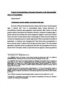
7. APPLICATION TO ENTITY BROWSING To demonstrate the actual usage of property clustering, we developed an online system called SView5. SView leverages property clustering to enhance the user experience of entity browsing in Linked Data. It groups and orders property-values of entities by their aspects for a neat presentation, and also offers various mechanisms for discovering related entities such as exploration based on link patterns and similarity-based entity recommendation. Moreover, users can personalize their browsing experience and they never work alone. They can consolidate entities following their own opinions, and their efforts are alleviated due to crowdsourced contributions from all users. Additionally, SView leverages users' contributions to generate global viewpoints on entity consolidation. Fig.1 shows the screenshot for viewing an entity “The Pentagon”6 in SView. Since this entity contains hundreds of property-values, it is not very readable if there is no appropriate organizing method. To address this issue, SView groups and orders property-values with aspects (e.g. “Building”), which reuse property clustering to identify closely related aspects of an entity and thus to help users capture related information quickly. A weighted set cover problem is formulated and solved to automatically pick up a small number of aspects that can cover as many relevant properties as possible.

We conducted user studies in SView to investigate how property clustering helps entity browsing. Specifically, we mainly focused on whether property clustering could help users find information of interest more quickly and the performance of different clustering algorithms. Figure 1. Screenshot for browsing entities in SView with property clustering

7.1. Baseline Approaches To demonstrate the effectiveness of different property clustering, we developed four approaches, including:  List: entity properties are organized into a flat list based on lexicographical ordering.  WordNet-based: entity properties are clustered based on the WordNet relatedness between property names ( RW ).  Co-occurrence-based: entity properties are clustered using the relatedness based on co-occurrence ( RU ).  Combination: entity properties are clustered based on a linear combination of WordNet-based relatedness and co-occurrence-based relatedness. The linear combination weights were both set to 0.5. For the latter three approaches, we leveraged the single linkage clustering algorithm to achieve property clustering results. The threshold of the single linkage algorithm was set as 0.3. For each cluster in the result, we used the domains of the properties in the cluster as the cluster's labels. We implemented these approaches in four prototypes. In all these prototypes, users could start browsing with an entity URI by entering into the input box. The entity description was presented in the center of the user interface. 7.2. Tasks We used the DBpedia and YAGO data sets in our experiment. We prepared the tasks as follows: We selected 10

classes (i.e. Athlete, Band, Building, Company, University, MusicalWork, Politician, PopulatedPlace, Software and River) according to the descending order of the number of instances of each class in DBpedia. Then, we selected one entity at random for each class. The tasks in browsing DBpedia entities are shown in Table 15. As to YAGO, we selected another 10 entities from YAGO in the same way. In total, we established 20 tasks to be used in our experiment. Table 15. Tasks for browsing DBpedia entities Question T1 T2 T3 T4 T5 T6 T7 T8 T9 T10

Entity

Find the debut Team, draft pick, draft round and draft year of Jeremy Shockey. Find the band member of Deep Purple. Find the build time and architect of Pentagon. Find the founding date, founder and the number of employees about Adobe systems. Find the number of students, staff and faculty about Bob Jones University. Find the producer, release date and sales amount about Load (album). Find the duty and tenure about Edmund Stoiber. Find the places near Somerset Calgary. Find the publisher and release date of Doom II. Find the length and source position of Tchefuncte River.

Jeremy_Shockey Deep_Purple The_Pentagon Adobe_Systems Bob_Jones_University Load_(album) Edmund_Stoiber Somerset,_Calgary Doom_II:_Hell_on_Earth Tchefuncte_River

7.3. Procedure The subjects consisted of 35 students majoring in computer science who were familiar with the Web, but with no knowledge of our project. The evaluation was conducted in three phases. First, the subjects learned how to use the given prototypes through a tutorial about 20 minutes, and had additional 10 minutes for free use and questions. After that, the subjects were given the tasks and responded to two pre-task questions about task context: PreQ1: I am familiar with the entity described in this task. PreQ2: I think it will be easy to complete this task. Second, each subject carried out 10 tasks by using randomly selected prototype per task. Though the task assignment was produced randomly, it was guaranteed that each subject took five tasks for DBpedia entities and five tasks for YAGO entities, and that each subject used every prototype exact two times. So, each prototype was used 70 times in total. Each subject was required to complete 10 tasks in 10 minutes. We recorded their answers, and the time that they spent on each task. With regard to each prototype, the subjects responded to the questionnaire about effectiveness: PostQ1: Rating about necessity of property clustering for browsing entity. PostQ2: Rating about usefulness of the prototype. Then, for each prototype, the subjects responded to the system usability scale (SUS) questionnaire. The questions in the two above questionnaires were responded by using a five-point Likert scale ranging from 1 (strongly disagree) to 5 (strongly agree). Finally, the subjects were asked to comment on the four prototypes. 7.4. Results 7.4.1. Task Context Pre-task questions in Table 16 capture subject-perceived task difficulty and entity familiarity. Repeated measures ANOVA revealed that the differences in subjects' mean ratings with different prototypes were not statistically significant (p>0.05), which supported that tasks were carried out with different prototypes in comparable contexts in terms of task difficulty and entity familiarity. So, these two factors are excluded from the following discussion. Table 16. Results of pre-task questions Response: Mean (SD)

F (p-value)

List WordNet Co-occurrence Combination PreQ1: 2.2 (1.095) 2.6 (1.303) 2.3 (1.119) 2.7 (1.442) 0.917 (0.456) PreQ2: 3.6 (0.932) 3.5 (1.225) 3.8 (0.997) 4.0 (0.788) 1.139 (0.340) 7.4.2. User Feedback Post-task questions capture subjects' experience with different approaches in Table 17. Repeated measures ANOVA revealed that the differences in subjects' mean ratings were all statistically significant (p List Table 18 summarizes SUS scores of different prototypes. Repeated measures ANOVA revealed that the difference in SUS score was statistically significant (p WordNet 7.4.3. Time Analysis Figure 2 shows the average time spent on the tasks in DBpedia and YAGO. In DBpedia, subjects required more time to complete these tasks, because each entity of these tasks in DBpedia had more properties than YAGO. With respect to different approaches, the Combination method outperformed other approaches. Co-occurrence had a better result than WordNet and List. 7.4.4. User Comments We summarized all the major comments that were made by at least five subjects. On List, 31 subjects (88.6%) said that there were no semantic relations among entity properties, and the large quantities of properties often made it difficult to retrieve interesting information. On WordNet, 20 subjects (57.1%) thought that it clustered the properties having semantic relatedness, but 12 subjects (34.3%) said that some clusters were too difficult to be understood, because some properties within these clusters are not semantically related. On Co-occurrence, 11 subjects (31.4%) said that it grouped the properties that were frequently used together, but 9 subjects (25.7%) thought that it had some potential risks, i.e. some clusters had too many properties. On the Combination, 33 subjects (94.3%) said that it provided a better clustering that had semantic similarity. 9 subjects (25.7%) claimed that the label of each clustering provided a better overview for entity description, but 16 subjects (45.7%) said that the labels were too difficult to be understood.

According to the above discussion, the Combination method can help users find information of interest more quickly and enhance user experience in entity browsing. Figure 2. Average consumption time per task

8. DISCUSSION OF FINDINGS The experimental results that we have shown allow us to answer our questions Q1 to Q4. This section discusses our findings from the obtained experimental results.  We empirically investigated 13 property relatedness measures that can be divided into five categories: lexical similarity between property names, semantic relatedness between property names, distributional relatedness between properties, domain/range relatedness between properties and overlap of property values. Different measures have different criteria for determining whether two properties are aspect-related. All these measures have different strengths and weaknesses and their performance may vary w.r.t. different clustering algorithms. Lexical similarity is very effective in property clustering, and the lexical similarity measures produce high precision (F-Score) results when property names share a large number of words or substrings. However, these measures fail to work when the number of shared words is small. By using a proper clustering algorithm, Jaro-Winkler ( RJ ) is preferable to the other lexical similarity measures in terms of Precision, and N-gram ( RN ) should be used when favoring F-Score. Semantic relatedness measures between property names are able to identify a large number of aspect-related properties by making use of the semantic relations of words from external knowledge sources. However, they may suffer from the limited coverage problem like WordNet, or suffer from noises due to the fact that their computation fails to consider the context of properties. ESA represents words as a weighted mixture of a predetermined set of natural concepts, which are defined by humans themselves and can be easily explained. When requiring for semantic relatedness between names, ESA is more recommended than WordNet or word embedding due to its larger coverage and higher quality. In addition, the graph embedding-based measure RG and the domain relatedness measure RD are appropriate for generating clusterings favoring high Recall.  We empirically evaluated seven clustering algorithms: DBSCAN ( CD ), single linkage ( CL ), complete linkage ( CC ), average linkage ( C A ), K-means ( CK ), spectral clustering ( CS ) and affinity propagation ( CP ). These algorithms have different criteria for clustering properties into meaningful groups and they perform differently on different relatedness measures. From the overall results, CD is similar to CL due to our parameter settings. Generally speaking, the density-based algorithm CD and the three hierarchical algorithms ( CL , CC and C A ) perform better than the other three CK , CS and CP in terms of Precision or F-Score on single measures. This may be due to the fact that the partition-based algorithms CK and CS





 







as well as CP perform poorly on non-spherical-shaped clusters like our sample dataset with large variance in sizes (Reddy & Vinzamuri, 2013). In this case, the density-based algorithm CD may be more suitable for our sample dataset since it is able to find any-shaped clusters. Among the density-based algorithm and the three hierarchical algorithms, DBSCAN ( CD ) and single linkage ( CL ) are more recommended to use in terms of F-Score. We empirically investigated two combination methods: the linear combination of measures and consensus clustering, by using different clustering algorithms. Both combination methods integrate the criteria of the complementary measures to generate better clustering results. However, they performed differently and achieved different results. The performance of consensus clustering is generally independent of the clustering algorithms used, since consensus clustering just takes the clustering results of single measures as input. Furthermore, consensus clustering only clusters together those strongly related properties that are identified by the majority of the results from single measures. As a result, no matter what clustering algorithm is used, consensus clustering always improves the Precision values of the clustering results compared to single measures. In other words, consensus clustering is preferable to high Precision results. Different from consensus clustering, the performance of linear combination of measures depends on the clustering algorithm used. This is because the linear combination of measures only provides the relatedness of properties, which is just the input of a clustering algorithm. The clustering result is finally generated by the clustering algorithm used. Thus, the criterion of the clustering algorithm for determining how properties are grouped together also affects the performance of linear measure combination in terms of Precision, Recall or F-Score. For example, linear combination is able to improve the Recall value used with the clustering algorithm CD , CL or C A , and improve the F-Score value used with CK or CS . Thus, the measures and clustering algorithm used in the linear combination need to be properly chosen for achieving clustering results of high Recall or F-Score. From the results of the user study on property clustering in entity browsing, we can see that, although not very high F-Score was obtained on the 40 sample entities, property clustering was still useful for helping user find information more quickly and enhancing the user experience during browsing entities. This is also the reason that several existing entity browsing systems consider manually clustering. In addition, in the user study, the users preferred the Combination method that was based on the linear combination of measures. It may be due to the reason that a user can find more related property information in a cluster for the tasks. The results of the user study showed the potentials of automatically clustering large-scale properties for entity browsing. However, there are some issues that have not been fully covered during our evaluation: There are not a few well-known clustering algorithms in the field of machine learning or data mining that we have not considered yet. In this paper, we selected several typical algorithms. Some sophisticated clustering algorithms adapted for our sample dataset may improve the our results. There also exist some relatedness measures between properties that have not been investigated in this study. It is possible that some of them may bring in performance change. Additionally, the computation of the distributional relatedness measures between properties is largely influenced by the underlying dataset. Making use of a more representative dataset may improve the clustering quality. Currently, the gold standard of property clustering was constructed by leveraging Freebase, while Freebase's division of properties does not consider the context of a specific entity. This may restrict the flexibility of experts when generating property clusterings and reduce the adaptability on a specific entity. The crowdsourcing technique can be used in the future to help build the gold standard at a large scale. The quality of linear combination relies on the clustering algorithm and the relatedness measures used. More investigations need to be performed to find the correlation between the linear combination, clustering algorithms and measures. Additionally, if a larger training dataset for property clustering can be constructed, we can perform linear or non-linear combinations of different measures by using various machine learning algorithms. In our sample dataset, the property clusterings have great variance in sizes and densities. As a result, there still exists a gap between the ideal clustering quality and the one achieved by the clustering algorithms that

we selected. This implies that more specific solutions need to be developed for property clustering in Linked Data. 9. CONCLUSION In this paper, we studied property clustering in Linked Data and evaluated 13 property relatedness measures, seven property clustering algorithms and two combination methods. Our experimental results demonstrated the feasibility of the automated property clustering. We also showed that property clustering can enhance entity browsing in practice. In addition, the generated property clusterings can be served as a benchmark or training data for the data mining and machine learning research. In future work, we will improve the quality of property clustering by leveraging crowdsourcing and active learning. We will also investigate more use scenarios for property clustering in Linked Data. ACKNOWLEDGMENT This research was supported by the National Natural Science Foundation of China (Nos. 61370019 and 61572247). We appreciate our students’ participation in the experiments. REFERENCES Abedjan, Z., & Naumann, F. (2013). Synonym analysis for predicate expansion. In P. Cimiano, O. Corcho, V. Presutti, L. Hollink, & S. Rudolph (Eds.), Proceedings of the 10th Extended Semantic Web Conference (pp. 140–154). Heidelberg: Springer. Ailon, N., Charikar, M., & Newman, A. (2008). Aggregating inconsistent information: Ranking and clustering. Journal of the ACM, 55 (5), 23:1–23:27. Bordes, A., Usunier, N., García-Durán, A., Weston, J., & Yakhnenko, O. (2013). Translating embeddings for modeling multi-relational data. In C. J. C. Burges, L. Bottou, Z. Ghahramani, & K. Q. Weinberger (Eds.), Proceedings of the 27th Conference on Neural Information Processing Systems (pp. 2787–2795). Curran Associates, Inc. Budanitsky, A., & Hirst, G. (2006). Evaluating WordNet-based measures of lexical semantic relatedness. Computational Linguistics, 32 (1), 13–47. Cheng, G., Gong, S., Li, X., Liu, Q., Zheng, L., Jiang, J., Hu, W., & Qu, Y. (2013). SView: Sharing views for browsing linked data. Online proceedings on the Semantic Web Challenge website. Cheng, G., & Qu, Y. (2013). Relatedness between vocabularies on the web of data: A taxonomy and an empirical study. Journal of Web Semantics, 20, 1–17. Evert, S. (2008). Corpora and collocations. In A. Lüdeling & M. Kytö(Eds.), Corpus linguistics: An international handbook (pp. 1212–1248). Berlin: Mouton de Gruyter. Fleiss, J. (1971). Measuring nominal scale agreement among many raters. Psychological Bulletin, 76 (5), 378– 382. Frey, B. J., & Dueck, D. (2007). Clustering by passing messages between data points. Science, 315, 972-977. Gabrilovich, E., & Markovitch, S. (2007). Computing semantic relatedness using wikipedia-based explicit semantic analysis. In M. M. Veloso (Ed.), Proceedings of the 20th International Joint Conference on Artificial

Intelligence (pp. 1606–1611). AAAI Press. Gong, S., Li, H., Hu, W., & Qu, Y. (2016). An empirical study on property clustering in linked data. In Y. Li et al. (Eds.), Proceedings of the 6th Joint International Semantic Technology Conference (pp. 67–82). Heidelberg: Springer. Gracia, J., & Mena, E. (2008). Web-based measure of semantic relatedness. In J. Bailey, D. Mairt, K.-D. Schewe, B. Thallheim, & X. S. Wang (Eds.), Proceedings of the 9th International Conference on Web Information Systems Engineering (pp. 136–150). Heidelberg: Springer. Gunaratna, K., Thirunarayan, K., & Sheth, A. P. (2015). FACES: diversity-aware entity summarization using incremental hierarchical conceptual clustering. In B. Bonet & S. Koenig (Eds.), Proceedings of the 29th AAAI Conference on Artificial Intelligence (pp. 116–122). AAAI Press. Hearst, M. A. (2006). Clustering versus faceted categories for information exploration. Communications of the ACM, 49 (4), 59–61. Hu, W., & Jia, C. (2015). A bootstrapping approach to entity linkage on the semantic web. Web Semantics: Science, Services and Agents on the World Wide Web, 34, 1–12. Isele, R., & Bizer, C. (2013). Active learning of expressive linkage rules using genetic programming. Journal of Web Semantics, 23, 1–15. Lin, D. (1998). An information-theoretic definition of similarity. In J. W. Shavlik (Ed.), Proceedings of the 15th International Conference on Machine Learning (pp. 296–304). San Francisco: Morgan Kaufmann. Lin, Y., Liu, Z., Sun, M., Liu, Y., & Zhu, X. (2015). Learning entity and relation embeddings for knowledge graph completion. In B. Bonet & S. Koenig (Eds.), Proceedings of the 29th AAAI Conference on Artificial Intelligence (pp. 2181–2187). AAAI Press. Mikolov, T., Sutskever, I., Chen, K., Corrado, G. S., & Dean, J. (2013). Distributed representations of words and phrases and their compositionality. In C. J. C. Burges, L. Bottou, Z. Ghahramani, & K. Q. Weinberger (Eds.), Proceedings of the 27th Conference on Neural Information Processing Systems (pp. 3111–3119). Curran Associates, Inc. Oren, E., Delbru, R., & Decker, S. (2006). Extending faceted navigation for RDF data. In I. F. Cruz et al. (Eds.), Proceedings of the 5th International Semantic Web Conference (pp. 559–572). Heidelberg: Springer. Quan, D., & Karger, D. (2004). How to make a semantic web browser. In S. I. Feldman, M. Uretsky, M. Najork, & C. E. Wills (Eds.), Proceedings of the 13th International Conference on World Wide Web (pp. 255– 265). New York: ACM. Reddy, C. K., & Vinzamuri, B. (2013). A survey of partitional and hierarchical clustering algorithms. In C. C. Aggarwal & C. K. Reddy (Eds.), Data clustering: Algorithms and applications (pp. 87–110). London: Chapman & Hall. Rutledge, L., van Ossenbruggen, J., & Hardman, L. (2005). Making RDF presentable: integrated global and local semantic web browsing. In A. Ellis & T. Hagino (Eds.), Proceedings of the 14th International Conference on World Wide Web (pp. 199–206). New York: ACM. Shvaiko, P., & Euzenat, J. (2013). Ontology matching: State of the art and future challenges. IEEE Transactions

on Knowledge and Data Engineering, 25 (1), 158–176. Smith, T., & Frank, E. (2016). Introducing machine learning concepts with weka. In E. Mathé& S. Davis (Eds.), Statistical genomics (pp. 353–378). Heidelberg: Springer. Wagner, S., & Wagner, D. (2007). Comparing clusterings: An overview (Tech. Rep.). Karlsruhe, Germany: Universität Karlsruhe, Fakultät für Informatik. Winkler, W. E. (1990). String comparator metrics and enhanced decision rules in the fellegi-sunter model of record linkage. In Proceedings of the Section on Survey Research Methods (pp. 354–359). Zhang, Z., Gentile, A. L., Blomqvist, E., Augenstein, I., & Ciravegna, F. (2013). Statistical knowledge patterns: Identifying synonymous relations in large linked datasets. In H. Alani et al. (Eds.), Proceedings of the 12th International Semantic Web Conference (pp. 703–719). Heidelberg: Springer. ENDNOTES 1 Corresponding author: Wei Hu ([email protected]) 2 https://drive.google.com/file/d/0B7XkCwpI5KDYNlNUTTlSS21pQmM/edit 3 http://km.aifb.kit.edu/projects/btc-2011 4 http://ws.nju.edu.cn/sview/propcluster_ijswis.zip 5 http://ws.nju.edu.cn/sview 6 http://dbpedia.org/resource/The_Pentagon Saisai Gong is a Ph.D. student at the Department of Computer Science and Technology, Nanjing University. He received his B.Sc. degree in Computer Science and Technology in 2009 and his M.Sc. degree in Computer Softw are and Theory in 2012, both from Southeast University. His research interests include Semantic Web, linked dat a browsing and data integration. Wei Hu is an associate professor at the Department of Computer Science and Technology, Nanjing University. He received his B.Sc. degree in Computer Science and Technology in 2005 and his Ph.D. degree in Computer Software and Theory in 2009, both from Southeast University. His research interests include Semantic Web, ontology engineering, data integration and biomedical knowledge discovery. Haoxuan Li is a Master student at the Department of Computer Science and Technology, Nanjing University. He received his B.Sc. degree in Computer Science and Technology from Nanjing University in 2016. His research interests include data integration and question answering. Yuzhong Qu is a full professor and Ph.D. supervisor at the Department of Computer Science and Technology, Nanjing University. He received his B.Sc. and M.Sc. degrees in Mathematics from Fudan University in 1985 and 1988 respectively, and his Ph.D. degree in Computer Software from Nanjing University in 1995. His research interests include Semantic Web, Web science and question answering.