generalized LVQ (GLVQ), and the soft nearest proto- type classifier ... class probability (MAXP) method [5], the soft near- ..... [8] S. Seo and K. Obermayer. Soft ...
Prototype Learning with Margin-Based Conditional Log-likelihood Loss Xiaobo Jin Cheng-Lin Liu Xinwen Hou National Laboratory of Pattern Recognition, Institute of Automation, Chinese Academy of Sciences 95 Zhongguancun East Road, Beijing 100190, P. R. China {xbjin,liucl,xwhou}@nlpr.ia.ac.cn Abstract The classification performance of nearest prototype classifiers largely relies on the prototype learning algorithms, such as the learning vector quantization (LVQ) and the minimum classification error (MCE). This paper proposes a new prototype learning algorithm based on the minimization of a conditional log-likelihood loss (CLL), called log-likelihood of margin (LOGM). A regularization term is added to avoid over-fitting in training. The CLL loss in LOGM is a convex function of margin, and so, gives better convergence than the MCE algorithm. Our empirical study on a large suite of benchmark datasets demonstrates that the proposed algorithm yields higher accuracies than the MCE, the generalized LVQ (GLVQ), and the soft nearest prototype classifier (SNPC).
1. Introduction Nearest neighbor classification is a simple and appealing non-parametric method for pattern classification. It does not need any preprocessing of the training data, but suffers from heavy burden of storage space and computation in classification. Prototype selection and prototype learning methods are efficient to reduce the number of prototypes and meanwhile improve the classification accuracy of nearest neighbor classifier (also called nearest prototype classifier). The well-known Learning Vector Quantization (LVQ) algorithm of Kohonen [4] offers intuitive and simple, yet powerful prototype learning rules in supervised learning. The LVQ algorithm yields superior classification performance although it does not guarantee convergence in training [7]. Crammer et al. [2] show that LVQ falls in a family of maximal margin learning algorithms and they present a rigorous bound on the generalization error of LVQ . Many other prototype learning algorithms based on
978-1-4244-2175-6/08/$25.00 ©2008 IEEE
loss minimization have been shown to give higher classification accuracies than LVQ [5]. These algorithms include the minimum classification error (MCE) method [3], the generalized LVQ (GLVQ) [7], the maximum class probability (MAXP) method [5], the soft nearest prototype classifier (SNPC) [8], etc. The MCE and GLVQ methods minimize margin-based loss functions, while the MAXP and SNPC formulate multiple prototypes in a Gaussian mixture framework and aim to minimize the Bayesian classification error on training data. The margin-based algorithms, including LVQ, MCE and GLVQ, only adjust two prototypes during one update. The training complexity of the MAXP and SNPC methods can be similarly decreased by pruning prototype updating according to the proximity of prototypes to the input pattern or the windowing rule. This paper proposes a new margin-based prototype learning algorithm, called log-likelihood of margin (LOGM). This algorithm is derived from the conditional log-likelihood loss (CLL), which is a convex function of the margin. The convex loss function leads to better convergence performance. A regularization term is added to the loss function for avoiding overfitting in training. The experimental results show that the LOGM algorithm gives higher test accuracies than the MCE, GLVQ and SNPC methods in most cases. Section 2 describes the framework of prototype learning algorithm as well as the MCE algorithm. Then Section 3 presents the LOGM algorithm and its regularization. Section 4 details some experiments and the conclusions are given in Section 5.
2. Prototype Learning Algorithm Let us consider a labeled data set D = {(xn , yn )|n = 1, 2, · · · , N }, where xn ∈ Rd and yn ∈ {1, 2, · · · , L} (L is the number of classes). The prototype learning algorithms design a set of prototypes {uls |s = 1, 2, · · · , S} for each class l (S can be different for different classes). The test pattern x
is classified to the class of the closest prototype. The choice of distance measure plays a crucial role in the algorithm performance but it is not on our focus. We only consider the Euclidean distance for simplicity. The expected Rrisk based on loss function φ is defined as Rφ f = φ(f (x)|x)p(x)dx where φ(f (x)|x) is the loss that x is classified by the decision f (x), and p(x) is the probability density at the sample point x. In practice, the empirical average loss on finite samples is comˆ φ f = 1 PN φ(f (xn )|xn ). Generally, puted by R n=1 N the loss function depends on the set of the prototype vectors Θ = {uls |l = 1, 2, · · · , L; s = 1, 2, · · · , S}. ˆ φ satisfies At the stationary point, the loss function R ˆ ∇Θ Rφ = 0. The prototypes are updated on each sample by gradient descent: Θ(t + 1) = Θ(t) − η(t)∇φ(f (x)|x)|x=xn ,
(1)
where η(t) is the learning rate of the algorithm in the t-th iteration. In MCE algorithm, φ(f ) is represented as the misclassification rate. When x with the genuine class l is classified, the misclassification rate is 1 − P (Cl |x). MCE algorithm aims to find the optimal parameters to minimize the misclassification rate on the training set by approximating the posterior probability P (Cl |x). The discriminant function for xn (k is the genuine class label) is given by: gk (xn ) = max{−kxn −uks k2 } = −kxn −uki k2 , (2) s
where k · k is the Euclidean metric. The misclassification measure [3] can be defined as follow: (3) dk (xn ) = −gk (xn ) + gr (xn ), where gr (xn ) = maxl6=k gl (xn ) = −kxn − urj k2 . We may view −dk (xn ) as the margin of xn which is similar to the hypothesis margin [2]. The misclassification loss of xn is approximated by a the sigmoid function σ(x): φ(xn ) = 1 − P (Ck |xn ) = 1 −
1 1 + eξdk (xn )
,
(4)
where ξ (ξ > 0) is a constant. It is easy to calculate the derivative of the loss as
uki
=
urj
=
which results in a perfect converge performance.
3. Conditional Log-Likelihood Loss for Prototype Learning 3.1. LOGM Algorithm Conditional Log-Likelihood Loss (CLL) is widely used in statistical pattern classification such as logistic regression. In general, the conditional likelihood function for multi-class is given by L N Y Y
P (T |Θ) =
P (Cl |xn )tnl ,
(8)
n=1 l=1
where tnl = I[xn ∈ Cl ] and I[x] is the indicator. Taking the negative logarithm then gives E=−
L N X X
tnl ln P (Cl |xn ),
(9)
n=1 l=1
which is known as Conditional Log-Likelihood Loss. The loss associated with xn is computed as: φ(xn ) = −
L X
tnl ln P (Cl |xn ).
(10)
l=1
For a pattern xn , we may view the genuine class of xn as the positive class and the remain classes as the negative class. Given that uki and urj are the closest prototype to xn in the positive class and in the negative class, respectively, we can define the discriminant function for a binary classification problem: f (xn ) = gk (xn ) − gr (xn ) = −dk (xn ).
(11)
Like MCE, the posterior probability can be approximated by the sigmoid function: 1 , (12) 1 + eξdk (xn ) where y = +1 since the posterior probability estimation is about the positive class (the genuine class k). Obviously, yf (x) is the margin of the pattern x. If yf (x) < 0, x is misclassified. We can obtain the following derivative: P (Ck |xn ) = σ(ξyf (xn )) =
∂φ(xn ) ∂φ(xn ) ∂φ(xn ) = −ξφ(xn )(1−φ(xn )), =− , ∂gki ∂grj ∂gki (5) where gki = −kxn − uki k2 and grj = −kxn − urj k2 . When the training pattern xn is given in the t-th iteration, two prototypes in class k and r are updated by: ∂φ(xn ) uki − 2η(t) (xn − uki ) ∂gki ∂φ(xn ) urj − 2η(t) (xn − urj ). ∂grj
In GLVQ [7], dk (xn ) is measured by the relative difference instead: −gk (xn ) + gr (xn ) , (7) dk (xn ) = gk (xn ) + gr (xn )
(6)
∂φ(xn ) ∂φ(xn ) ∂φ(xn ) = −(1 − P (Ck |xn ))ξ, =− . ∂gki ∂grj ∂gki (13) Two prototypes are updated by (6) when the training pattern xn with the genuine class k is given.
3.2. Regularization of Prototype Learning Algorithms The minimization of misclassification loss may lead to unstable solutions. Unlike that the maximization of sample margin (for support vector machines, e.g.) is beneficial to the generalization performance, the enlarging of hypothesis margin may deteriorate the generalization performance. To constrain the hypothesis margin of MCE and LOGM algorithms, we add a regularization term to the loss function in a similar way of [6]: ˜ n ) = φ(xn ) + αkxn − uki k2 , φ(x
(14)
where α is the regularization coefficient. Institutively, the regularizer makes the winning prototype move toward xn . The prototypes now are updated by
Figure 1. The loss of MCE and LOGM algorithm based on the margin yf (x)
∂φ(xn ) − α)(xn − uki ) ∂gki ∂φ(xn ) − 2η(t) (xn − urj ). (15) ∂grj
uki
=
uki − 2η(t)(
urj
=
urj
For fair comparison, we also add a regularization term in the SNPC algorithm [8]: X ˜ n ) = φ(xn ) − α log( exp(ξgkj )), (16) φ(x j
P where φ(xn ) = 1 − Pk (xn ) and Pl (xn ) = s Pls (xn ) ls (xn )) given Pls (xn ) = Pexp(ξg . The second term exp(ξg (x )) i,j
ij
n
is the negative log-likelihood of the class-conditional density about the positive class, which makes all prototypes in the positive class move toward xn with the (xn ) . Then the prototypes are updated by ratio PPlsk (x n) uls
uls
φ(xn ) (xn − uls ) gls Pls (xn ) (xn − uls ), l = k +2η(t)αξ Pk (xn ) φ(xn ) = uls − 2η(t) (xn − uls ), l 6= k,(17) gls =
uls − 2η(t)
where s = 1, 2, · · · , S and the derivative of the loss function is as follow: ½ ∂φ(xn ) −ξPls (xn )(1 − Pk (xn )), l = k; = ξP l 6= k. ∂gls ls (xn )Pk (xn ), (18)
3.3. Discussions The margin-based prototype learning algorithms aim to minimize different loss functions based on certain margin. MCE and LOGM optimize the loss
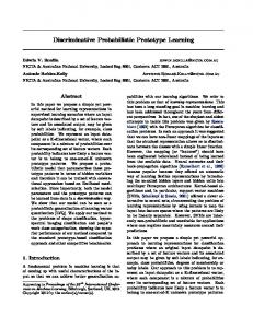
Figure 2. Average margins of different algorithms during training on the USPS dataset with S = 20 and α = 0.001 (x))) 1 and ln (1+expln(−yf , respectively. 2 The loss functions are plotted in Figure 1 where yf (x) = gk (x)−gr (x) . The property of classificationcalibration [1] about two losses guarantees that the minimization of Rφ (f ) may provide a reasonable surrogate for the minimization of 0-1 loss. The strictness of convexity about the loss of LOGM avoids running into the ˆ φ (f ∗ ) local optimal point and obtains more optimal R risk. Figure 2 demonstrates average margins of different algorithms on the USPS dataset during learning. We see that after 100 iterations LOGM can obtain larger average margin than MCE and GLVQ on the regularization condition. 2 1+exp (2yf (x))
4. Experiments We compare the performance of the proposed LOGM with other three representative prototype learning algorithms (MCE, SNPC and GLVQ) on 10 small 1 Two
loss functions are scaled to pass through the point (0, 1)
UCI benchmark data-sets 2 and 2 large datasets which include USPS and 20NG (20newgroups) listed in Table 1. Each example of USPS is a 256-dimensional vector with entries between 0 and 255. The 20NG dataset is a collection of approximately 20,000 documents that were collected from 20 different newsgroups 3 .The bydate version of this data set along with its train/test split was used in our experiments for the convenience of comparisons. The information gain method was used for selecting 1,000 highest score features. In implementing the algorithms, the prototypes were initialized by K-means clustering of classwise data. The initial learning rate η(0) was set to 0.1τ ∗ cov, where τ was drawn from {0.1, 0.5, 1, 1.5, 2} and cov is the average distance of all training patterns to the nearest cluster center. In the t-th iteration, the learning +n rate of the n-th pattern was η(0)(1 − tN T N ), where T is the maximum iteration time. For 10 small UCI datasets, T was set to 100 and the prototype number S was set to {1, 2, 3, 4, 5}. For USPS and 20NG, T was set to 40 and S was set to {5, 10, 15, 20, 25} following [4]. The regularization coefficient α was set to {0, 0.001, 0.005, 0.01, 0.05}. The training parameters and model parameters could be optimized in the space of the cubic grid (α, S, τ ) by cross-validation on the training data. All experiments ran on the framework of Torch 4 , a C++ library. In 10 small data-sets, the accuracy of an algorithm on a data set was obtained via 10 runs of ten-fold cross validation. Runs of the various algorithms were carried out on the same training sets and evaluated on the same test sets. About 1/3 of the training data-set were used for the validation of hyper-parameters. But for USPS and 20NG, we only chose 1/5 of the training examples for validation. Then all of the training data-set were retrained under the optimal hyper-parameters. Table 1 gives the accuracies and the standard deviations of different prototype learning algorithms. For USPS and 20NG, the validation parameters (α, S, τ ) are included in the brace. The positivity of α shows that the regularization technique benefits the performance of prototype learning. We see LOGM gives the highest accuracy on 7 of 12 data-sets. In the difficult datasets glass2 and vehicle, the advantage of LOGM is remarkable. We use sign-rank test to compare LOGM with other algorithms in the statistical significance. It is found that LOGM is more superior than MCE (p = 0.1099), SNPC (p = 0.1099) and GLVQ (p = 0.0640). The p-value shows the significance probability of no difference between two algorithms. 2 http://www.ics.uci.edu/mlearn/MLRepository.html 3 http://people.csail.mit.edu/jrennie/20Newsgroups/ 4 http://www.torch.ch/
Table 1. Classification results: Empirical accuracy of the algorithms in [%] with standard deviation.
5. Conclusion and Further Research We have proposed a prototype learning algorithm (LOGM) based on the minimization of conditional loglikelihood loss and discuss its relations with MCE algorithm. A regularization term is added to avoid overfitting in training. In experiments on a large suite of benchmark datasets, LOGM is demonstrated to outperform the previous methods MCE,GLVQ and SNPC.
6. Acknowledgements This work is supported by the National Natural Science Foundation of China (NSFC) under grant no.60723005.
References [1] P. L. Bartlett, M. I. Jordan, and J. D. McAuliffe. Convexity, classification, and risk bounds. Journal of the American Statistical Association, 101(473):138–156, 2006. [2] K. Crammer, R. Gilad-Bachrach, A. Navot, and N. Tishby. Margin analysis of the lvq algorithm. In NIPS, pages 462–469, 2002. [3] B.-H. Juang and S. Katagiri. Discriminative learning for minimum error classification. IEEE Transactions on Signal Processing, pages 3042–3054, 1992. [4] T. Kohonen, J. Hynninen, J. Kangas, J. Laaksonen, and K. Torkkola. Lvq pak: The learning vector quantization program package. Technical report, Helsinki University of Technology, 1995. [5] C.-L. Liu and M. Nakagawa. Evaluation of prototype learning algorithms for nearest-neighbor classifier in application to handwritten character recognition. Pattern Recognition, 34(3):601–615, 2001. [6] C.-L. Liu, H. Sako, and H. Fujisawa. Discriminative learning quadratic discriminant function for handwriting recognition. IEEE Transactions on Neural Networks, 15(2):430–444, 2004. [7] A. Sato and K. Yamada. Generalized learning vector quantization. In NIPS, pages 423–429, 1995. [8] S. Seo and K. Obermayer. Soft learning vector quantization. Neural Computation, 15(7):1589–1604, 2003.