Semantic Subspace Learning with Conditional Significance Vectors Nandita Tripathi, Stefan Wermter, Chihli Hung, and Michael Oakes Abstract — Subspace detection and processing is receiving more attention nowadays as a method to speed up search and reduce processing overload. Subspace Learning algorithms try to detect low dimensional subspaces in the data which minimize the intra-class separation while maximizing the inter-class separation. In this paper we present a novel technique using the maximum significance value to detect a semantic subspace. We further modify the document vector using conditional significance to represent the subspace. This enhances the distinction between classes within the subspace. We compare our method against TFIDF with PCA and show that it consistently outperforms the baseline with a large margin when tested with a wide variety of learning algorithms. Our results show that the combination of subspace detection and conditional significance vectors improves subspace learning.
I. INTRODUCTION Many learning algorithms do not perform well with highdimensional data due to the curse of dimensionality [1]. Additional dimensions spread out the points making distance measures less useful. In very high dimensions, objects in a dataset are nearly equidistant from each other. Therefore, methods are needed that can discover clusters in various subspaces of high dimensional datasets [2]. Subspace learning methods are therefore nowadays being increasingly researched and applied to web document classification, image recognition and data clustering. Among subspace learning methods, Principal Component Analysis (PCA) [3] and Linear Discriminant Analysis (LDA) [4] are well known traditional methods. LDA is a supervised method whereas PCA is unsupervised. Other methods include ISOMAP, Locally Linear Embedding (LLE), Neighborhood Preserving Embedding (NPE), Laplacian Eigen Maps, Nonparametric Discriminant Analysis, Marginal Fisher Final Manuscript received April 26,2010. Nandita Tripathi is with the Department of Computing, Engineering and Technology, University of Sunderland, St Peters Way, Sunderland SR6 0DD, United Kingdom (e-mail: bf39rv@ student.sunderland.ac.uk) Stefan Wermter is with Institute for Knowledge Technology, Department of Computer Science, University of Hamburg, Vogt Koelln, Str. 30, 22527 Hamburg , Germany (e-mail:
[email protected]) Chihli Hung is with the Department of Information Management, Chung Yuan Christian University, Chung-Li, Taiwan 32023 R.O.C. (email:
[email protected]) Michael Oakes is with the Department of Computing, Engineering and Technology, University of Sunderland, St Peters Way, Sunderland SR6 0DD, United Kingdom (e-mail:
[email protected]).
Analysis and Local Discriminant Embedding [5]. Furthermore, the Supervised Kampong Measure (SKM) [6] is an incremental subspace learning method. The objective of all these algorithms is to minimize the intra-class distance while maximizing the inter-class separation. However, as the number of feature dimensions increases, the computational complexity for these algorithms increases dramatically. For instance, the computational complexity of PCA is O(p2n )+O(p3) where p is number of data dimensions and n is the number of data points [7]. In other approaches, Wang et al [8] use an RD-Quadtree to subdivide the data space and show that their RD–Quadtree-based clustering algorithm has better results for high-dimensional data than the wellknown K–means algorithm. Finally, Hinton & Salakhutdinov [9] have proposed the concept of Semantic Hashing where documents are mapped to memory addresses in such a way that semantically similar documents are located at nearby addresses. The majority of these methods have high computational complexity and as such cannot quickly focus the search when the amount of data is very large. We present here a novel method of subspace detection and show that it improves learning without lengthy computations. We use the semantic significance vector [10], [11] to incorporate semantic information in the document vectors. We compare the performance of these vectors against that of TFIDF vectors. The dimensionality of TFIDF vectors is reduced using PCA to produce a vector length equal to that of the semantic significance vectors. Our experiments were performed on the Reuters corpus (RCV1) using the first two levels of the topic hierarchy. Our method achieves the objective of the other subspace learning algorithms i.e. decreasing intra-class distance while increasing inter-class separation but without the associated computational cost. Subspace detection is done in O(k) time where k is the number of level 1 topics and thus can be very effective where time is critical for returning search results. II. METHODOLOGY OVERVIEW AND OVERALL ARCHITECTURE The topic codes in the Reuters Corpus [12] represent the subject areas of each news story. They are organized into four hierarchical groups, with four top-level nodes: Corporate/Industrial (CCAT), Economics (ECAT), Government/Social (GCAT) and Markets (MCAT). Under each top-level node there is a hierarchy of codes,
with the depth of each represented by the length of the code. Ten thousand headlines along with their topic codes were extracted from the Reuters Corpus. These headlines were chosen so that there was no overlap at the first level categorization. Each headline belonged to only one level 1 category. At the second level, since most headlines had multiple level 2 subtopic categorizations, the first subtopic was taken as the assigned subtopic. Thus each headline had two labels associated with it – the main topic (Level 1) label and the subtopic (Level 2) label. Headlines were then pre-processed to separate hyphenated words. Dictionaries with term frequencies were generated based on the TMG toolbox [13]. These were then used to generate the Semantic Significance Vector representation [10], [11] for each document. Two different variations of vector representations were used – the Full Significance Vector representation and the new Conditional Significance Vector representation. Masking of the vector elements was done by setting them to zero value. Different levels of masking were examined to generate a total of five different datasets. Each dataset
Training Document Set
Test Document Set
The WEKA machine learning workbench [14] was used to examine this architecture and representations with various learning algorithms. Ten algorithms were compared for our representations to examine the different categories of classification algorithms. Classification Accuracy, which is a comparison of the predicted class to the actual class, was recorded for each experiment run. III. STEPS FOR DATA PROCESSING AND DATA GENERATION FOR EXPERIMENTS 3.1 Text Data Preprocessing 10,000 Reuters headlines were used in these experiments. The Level 1 categorization of the Reuters Corpus divides the data into four main topics. These main topics and their distribution in the data along with the number of subtopics of each main topic in this data set are given in Table 1. Level 2 categorization further divides these into subtopics. Here we took the direct (first level nesting) subtopics of each main topic occurring in the 10,000 headlines. A total of 50 subtopics were included in these experiments. Some of these subtopics with their numbers present are shown in Table 2. Since all the headlines had multiple subtopic assignment e.g. C11/C15/C18, only the first subtopic e.g. C11 was taken as the assigned subtopic.
Document Significance Vector Generation 54 column document vector Subspace Detection 12 column (average value) subspace document vector
Learning Algorithm
Classification Decision Fig 1. Semantic Subspace Learning Architecture was then randomised and divided into two equal sets for training and testing, each comprising of 5000 document vectors. Fig 1 shows the semantic subspace learning architecture.
Table 1: Reuters Level 1 Topics No
Main Topic
Description
Number Present
No. of Subtopics
1
CCAT
Corporate/ Industrial
4600
18
2
ECAT
Economics
900
8
3
GCAT
Government/ Social
1900
20
4
MCAT
Markets
2600
4
Table 2: Some Reuters Level 2 subtopics used for our experiments. Main Topic
Sub Topic
Description
Number Present
CCAT
C17
Funding/ Capital
CCAT
C32
Advertising/ Promotion
10
CCAT
C41
Management
130
ECAT
E12
Monetary/ Economic
107
ECAT
E21
Government Finance
377
ECAT
E71
Leading Indicators
87
GCAT
G15
European Community
38
GCAT
GPOL
Domestic Politics
197
GCAT
GDIP
International relations
215
GCAT
GENV
Environment
30
MCAT
M11
Equity Markets
MCAT
M14
Commodity Markets
377
3.3 Data Sets Generation 617 1050
3.2 Semantic Significance Vector Generation We use a vector representation which looks at the significance of the data and weighs different words according to their significance for different topics. References [10] and [11] have introduced the concept of semantic significance vectors. Significance Vectors are determined based on the frequency of a word in different semantic categories. A modification of the significance vector called the semantic vector uses normalized frequencies. Each word w is represented with a vector (c1,c2,..,cn) where ci represents a certain semantic category and n is the total number of categories. A value v(w, ci) is calculated for each element of the semantic vector as the normalized frequency of occurrences of word w in semantic category ci (the normalized category frequency), divided by the normalized frequency of occurrences of the word w in the corpus (the normalized corpus frequency):
v( w, ci ) =
is simply referred to as Significance Vector. The TMG Toolbox [13] was used to generate the term frequencies for each word in each headline. The word vector consisted of 54 columns for 4 main topics and 50 subtopics. While calculating the significance vector entries for each word, its occurrence in all subtopics of all main topics was taken into account - hence called Full Significance Vector. We also generated vectors to observe whether results obtained with Full Significance can be improved by modifying the significance vectors to reflect the subspace which is being processed. Here again the word vector consisted of 54 columns for 4 main topics and 50 subtopics. However, while calculating the significance vector entries for each word, its occurrence in all subtopics of only a particular main topic was taken into account - henceforth called Conditional Significance Vector.
Normalised Frequency of w in ci ∑ Normalised Frequency of w in ck k
where k ∈ {1..n} For each document, the document semantic vector is obtained by summing the semantic vectors for each word in the document and dividing by the total number of words in the document. This is the version of the semantic significance vector used in our experiments. Henceforth it
As will be described below, datasets for five different vector representations were generated. The Full Significance Vectors were processed in different ways to generate four different data sets. The fifth set was the Conditional Significance Vector dataset. 3.3.1 No Mask Full Significance Data Set For each vector the first four columns, representing four main topics – CCAT, ECAT, GCAT & MCAT, were ignored leaving a vector with 50 columns representing 50 subtopics. The order of the data vectors was then randomised and divided into two sets – training set and testing set of 5000 vectors each. 3.3.2 Mask 1 Full Significance Data Set For each vector the numerical entries in the first four columns, representing four main topics – CCAT, ECAT, GCAT & MCAT, were compared. The topic with the minimum numerical value entry was identified. Then the entries for all subtopics belonging to this main topic were masked i.e. set to zero. Finally, the first four columns representing four main categories were deleted. The resultant vector had 50 columns representing 50 subtopics but the subtopic entries for the topic with least significance value had been masked to zero. The average number of relevant columns was then 38. The dataset was then randomised and divided into two sets – training set and testing set of 5000 vectors each. 3.3.3 Mask 2 Full Significance Data Set As above, the numerical entries in the first four columns of each vector representing four main topics CCAT,
ECAT, GCAT and MCAT were compared. The main topics with the two smallest numerical value entries were identified. Then the entries for all subtopics belonging to these two main topics were masked i.e. set to zero. Then, the first four columns representing four main categories were ignored. The resultant vector had 50 columns representing 50 subtopics but the subtopic entries for the two topics with the two smallest significance values had been masked to zero. The average number of relevant columns in this case became 25. The masked dataset was then randomised and divided into training and testing sets of 5000 vectors each. 3.3.4 Mask 3 Full Significance Data Set Here again, the numerical entries in the first four columns, representing four main topics – CCAT, ECAT, GCAT & MCAT, were compared. The topics with the three smallest numerical value entries were identified. Then the entries for all subtopics belonging to these three topics were masked i.e. set to zero. Finally, the first four columns representing four main categories were deleted. The resultant vector had 50 columns representing 50 subtopics but the subtopic entries for the three main topics with least significance value, 2nd least significance value and 3rd least significance value had been masked to zero. Since there are four main topics in the Reuters corpus, this has the same effect as allowing only the subtopics of the main topic with the maximum significance value in the resultant vector while masking out all the rest. The average number of relevant columns here was 12. Again the dataset was randomised and divided into training set and testing set of 5000 vectors each. 3.3.5 Mask 3 Conditional Significance Data Set In this case, while calculating the significance vector entries for each word in a subtopic, its occurrence in all subtopics of only a particular main topic was taken into account - hence called conditional significance vector. Here, when calculating significance values for C11, C12, etc, the topics considered were only the subtopics of CCAT. Similarly for M11, M12, etc only MCAT subtopics were considered. For each word, four separate conditional significance sub-vectors were generated for the four main Reuters topics. These sub-vectors were then concatenated together along with the significance value entries for the four main topics to form the 54 column word vector. The Conditional Significance document vector was generated by summing the conditional significance word vectors for each word appearing in the document and then dividing by the total number of words in the document. This vector representation is used to measure the significance of a word within a particular main topic. Hence only the subtopic entries for the main topic with maximum value entry were allowed. All the subtopic entries belonging to the other 3 main topics were masked out. The dataset was then randomised and divided
into two sets – training set and testing set of 5000 vectors each.
0
. . . . . 0 0.13 0.02 0.43 0.06 0.24
Full Document space
Subspace
0 . . . . 0
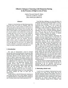
Fig 2: Mapping of Conditional Significance Vector to relevant subspace. Fig 2 shows the conceptual diagram for the conditional significance vector while Fig 3 shows the Conditional Significance Vector (CSV) for two different Reuters headlines. The Mask 3 Full Significance Vector (FSV) and Conditional Significance Vector (CSV) values for each of these two headlines are given below for comparison. The main topic label and subtopic label are shown at the end of each vector. As can be seen, the vector entries are boosted in the case of CSV – thus helping to differentiate between subtopics within the subspace Headline 1 0......0,0.20,0.03,0.04,0.02, MCAT/M11 : FSV 0......0,0.59,0.11,0.20,0.08, MCAT/M11 : CSV Headline 2 0….0,0.03,0.05,0.04,0.0099,0.01,0.0073, 0.25,0.0069, 0.....0,ECAT/E51 : FSV 0….0,0.13,0.13,0.10,0.0100,0.02,0.0300,0.52,0.0300, 0….0,ECAT/E51 : CSV
0 . . . . . . . . . . . . . 0 0.59 0.11 0.20 0.08
Label : M11 (MCAT)
Label : E51 (ECAT)
CCAT
CCAT
ECAT
ECAT
GCAT GCAT
MCAT MCAT
CSV Vector 1
0 . . 0 0.13 0.13 0.10 0.01 0.02 0.03 0.52 0.03 0 . . . . . . 0
Table 3: Classification Algorithms and their default parameters in Weka No.
Algorithm
Parameters
1.
Random Forest
NumTrees = 10
2.
J48 (C4.5)
Confidence factor=0.25, MinNumObj=2, NumFolds=3, Subtree raising =true
3.
Bagging
BagSizePerc=100, NumIterations=10, BaseClasifier=REP Tree
4.
Classification Regression
5.
LogitBoost
NumIterations =10, NumRuns =1, Shrinkage =1.0, Weight threshold =100, BaseClassifier = DecisionStump
6.
PART
Confidence factor=0.25, MinNumObj=2, NumFolds=3
7.
IBk
Knn=1, No cross validation, No distance weighting
8.
BayesNet
Estimator=SimpleEstimator, Search algorithm=K2
9.
NNge
NumAttemptsGeneOption=5 NumFoldersMIOption=5
Multilayer Perceptron
LearningRate=0.3, Momentum=0.2, Training time=500, RandomValidation threshold=20
CSV Vector 2
Fig 3: Conditional Significance Vectors showing nonzero entries for relevant subspace 3.4 TFIDF Vector generation The TMG toolbox [13] was used to generate TFIDF vectors for the ten thousand Reuters headlines used in these experiments. Dimensionality reduction was done using PCA with the same toolbox. The number of dimensions was chosen as 50 for PCA to have vectors similar in size to the significance vectors generated earlier. The dataset was then randomized and divided into two sets - training and test of 5000 vectors each. 3.5 Classification Algorithms Ten Classification algorithms were tested with our datasets namely Random Forest, C4.5, Bagging, LogitBoost, Classification via Regression, Multilayer Perceptron, BayesNet, IBk, NNge and PART. Random forests [15] are a combination of tree predictors such that each tree depends on the values of a random vector sampled independently. C4.5 [16] is an inductive tree algorithm with two pruning methods : subtree replacement and subtree raising. Bagging [17] is a method for generating multiple versions of a predictor and using these to get an aggregated predictor. LogitBoost [18] performs classification using a regression scheme as the base learner, and can handle multi-class problems. In Classification via Regression [19], one regression model is built for each class value. Multilayer Perceptron [20] is a neural network which uses backpropagation for training. BayesNet [21] implements Bayes Network learning using
10.
via
Classifier=M5P
various search algorithms and quality measures. IBk [22] is a k-nearest neighbour classifier which can select an appropriate value of k based on cross-validation and can also do distance weighting. NNge [23] is a nearest neighbor like algorithm using non-nested generalized exemplars (which are hyperrectangles that can be viewed as if-then rules). A PART [24] decision list uses separate-and-conquer. It builds a partial C4.5 decision tree in each iteration and makes the best leaf into a rule. Table 3 shows the different classification algorithms used with their default parameters in Weka.
All these algorithms can cope with different sized categories. This takes care of the different number of instances present for each category in Table 1. IV. RESULTS AND ANALYSIS Two sets of experiments were run to test learning at the first two levels of Reuters topic categorization. Ten runs of each algorithm with different seed values (wherever applicable) were taken for each vector representation. Four algorithms (Classification via Regression, IBk, BayesNet and NNge) did not have the option for entering a random seed value in Weka. Three algorithms (C4.5, LogitBoost and PART) had an option for entering random seed value but the results for all 10 runs were identical. Only three algorithms (Random Forest, Bagging and Multilayer Perceptron) showed variance in the classification accuracy values. The average and variance of the classification accuracy for 10 runs with different seed values was calculated for each algorithm. The abbreviations for the various options are given below:
Table 4a: Main Topic Average Classification Accuracy (%) for test vectors Bold Font (big) – best performance; Bold Font (small) 2nd best performance *No.
FS_0
FS_1
FS_2
FS_3
CS_3
TFIDF/ PCA 79.46
1.
91.17
90.67
91.45
96.45
2.
92.46
91.02
92.40
95.72
96.45 96.10
3.
92.24
91.95
93.54
96.39
96.29
78.89
4.
92.10
94.94
94.72
96.28
92.30
92.22
90.96
96.24
96.78 96.38
77.54
5. 6.
73.58
72.20
93.46
92.86
92.20
95.92
95.60
74.14
7.
96.84
96.74
95.28
95.44
95.94
76.74
8.
83.58
81.26
71.70
96.26
96.30
59.62
9.
95.66
95.58
89.92
96.64
96.34
73.72
10.
96.54
96.40
95.31
96.49
97.43
79.77
*Algorithm No FS_0: Full Significance with No Mask FS_1: Full Significance with Mask 1 FS_2: Full Significance with Mask 2 FS_3: Full Significance with Mask 3 CS_3: Conditional Significance with Mask 3 TFIDF/PCA: TFIDF with PCA reduction
Table 4b: Main Topic Classification Accuracy Variance for test vectors Bold Font (big) – best performance *No. 1.
The Algorithm Index is as follows: 1. Random Forest 2. J48 (C4.5) 3. Bagging 4. Classification via Regression 5. LogitBoost 6. PART 7. IBk 8. BayesNet 9. NNge 10. Multilayer Perceptron
2. 3. 4. 5. 6. 7. 8. 9. 10.
FS_0
FS_1
FS_2
FS_3
CS_3
TFIDF/ PCA
0.227
0.236
0.123
0.018
0.011
0.120
0
0
0
0
0
0
0.234
0.084
0.042
0.003
0.003
0.224
0
0
0
0
0
0
0
0
0
0
0
0
0
0
0
0
0
0
0
0
0
0
0
0
0
0
0
0
0
0
0
0
0
0
0
0
0.109
0.115
0.095
0.062
0.042
0.742
*Algorithm No 4.1 Level 1 Testing The Full Significance Vector with four variations – No Mask, Mask 1, Mask 2 and Mask 3 and the Conditional Significance Vector with Mask 3 were used with only the main topic labels i.e. CCAT, ECAT, GCAT and MCAT. The TFIDF/PCA vectors with main topic labels were used for comparison. The algorithms given above were run using 5000 training vectors and 5000 test vectors for each case. Table 4a shows the average accuracy values while Table 4b shows the variance in accuracy values for the test cases.
In Table 4a, all algorithms except IBk (No. 7) show that the maximum masking option (Mask 3) gives the best result. This indicates that the maximum significance value is a good indicator of the relevant subspace. The best results are divided between FS_3 and CS_3 for different algorithms. Table 4b shows that the minimum variance is also given by the maximum masking option (Mask 3). The best result is given by CS_3.
Table 5a: Subtopic Average Classification Accuracy (%) for test vectors Bold Font (big) – best performance; Bold Font (small) 2nd best performance *No.
FS_0
FS_1
FS_2
FS_3
CS_3
TFIDF/ PCA
82.11 87.90
80.69 87.62
74.69 78.50
88.55 88.90
90.60 90.42
57.37 49.16
4.
86.68 92.12
87.04 91.94
79.51 83.32
89.53 91.36
57.51 56.02
5.
92.32
92.10
83.88
91.16
6.
87.18
87.98
77.20
88.78
7.
90.84
90.58
81.76
89.66
8.
68.52
61.98
52.18
86.84
9.
91.30
91.16
82.34
90.96
92.06 92.98 92.62 90.24 91.22 89.04 92.42
91.96
91.86
82.07
91.39
92.39
58.84
1. 2. 3.
10.
52.98 50.44 55.52 46.74 54.82
*Algorithm No
Table 5b: Subtopic Classification Accuracy Variance for test vectors Bold Font (big) – best performance *No.
FS_0
FS_1
FS_2
FS_3
CS_3
TFIDF/ PCA
1.
0.545
1.239
0.264
0.101
0.146
0.202
2.
0
0
0
0
0
0
3.
0.233
0.241
0.151
0.030
0.028
0.147
4.
0
0
0
0
0
0
5.
0
0
0
0
0
0
6.
0
0
0
0
0
0
7.
0
0
0
0
0
0
8.
0
0
0
0
0
0
9.
0
0
0
0
0
0
10.
0.141
0.163
0.746
0.026
0.059
0.320
*Algorithm No
4.2 Level 2 Testing Here, the Full Significance Vector with four variations – No Mask, Mask 1, Mask 2 and Mask 3 and the Conditional Significance Vector with Mask 3 were used with the subtopic labels. The TFIDF/PCA vectors with subtopic labels were used for comparison here. The same algorithms as given above were run using 5000 training vectors and 5000 test vectors for each case. The results shown in Table 5a are the average accuracy values for the test cases. This subtopic accuracy table shows the
accuracy values obtained by applying classification algorithms after subspace branching. So this is a combined performance of level 1 and level 2. The Conditional Significance Vector representation with maximum masking option (Mask 3) gives the best average accuracy result with all algorithms. Table 5b shows that the minimum variance is again given by the maximum masking option (Mask 3). The best variance values are split between FS_3 and CS_3 here. The Mask 3 option consistently shows the best results at level 1 and level 2. This shows that the maximum significance value is successful in identifying the relevant subspace (level 1 topic). Since the Conditional Significance Vector with Mask 3 option encodes the subspace within the vector itself, the subtopic accuracy table shows the combined effect of branching at level one and applying the classification algorithms at level 2. Consistent maximum accuracy obtained at level 2 by the conditional significance vector with all the algorithms shows that conditional significance is successful in differentiating between subtopics within a data subspace. Thus our vector representation is unique in that it incorporates both subspace branching and subspace learning in the same step. V. CONCLUSION This work is an effort to explore semantic subspace learning with the overall objective of improving document retrieval in a vast document space. Our experiments on the Reuters Corpus show that the maximum significance value has potential in identifying the main (Level 1) topic of a document. They also show that modifying the significance vector (conditional significance) to process only the subspace improves learning within the subspace. Thus the combination of branching on maximum significance value along with using conditional significance improves subspace learning. The subspace detection is done by processing a single document vector. This method is independent of the total number of data samples and only compares the level 1 topic entries. The time complexity is thus O(k) where k is the number of level 1 topics. The novelty of our approach is in the vector representation. In the document conditional significance vector generated by the subspace detection step, the subspace is encoded in the vector (the non-zero values represent the subspace). Secondly, the numerical significance values in the word conditional significance vector denote the significance of a particular word for different subtopics within that subspace. Since the document vector is a summation of the word vectors, this helps in differentiating between topics within a given subspace (between subtopics of a main topic in case of Reuters Corpus) thus enhancing subspace learning. In this work, the word significance vectors were calculated using only term frequencies. For further work, the effect of a
global weighting measure like Inverse Document Frequency (IDF) on the word weights can be explored. REFERENCES [1] [2] [3] [4] [5] [6]
[7]
[8]
[9] [10]
[11] [12]
[13]
[14]
[15] [16] [17] [18] [19] [20] [21]
J.H. Friedman,“On Bias, Variance, 0/1—Loss, and the Curse-ofDimensionality,” In Data Mining and Knowledge Discovery, Volume 1, Issue 1, 1997, pp 55 - 77 L. Parsons, E. Haque & H. Liu, “Subspace Clustering for High Dimensional Data : A Review,” In ACM SIGKDD Explorations Newsletter, Vol 6, Issue 1, 2004, pp 90 – 105 I. Joliffe , “Principal Component Analysis,” New York: Springer-Verlag, 1986 K. Fukunaga, “Introduction to statistical pattern recognition,” 2nd edition , Academic Press, New York, 1990. J.Yang, S.Yan & T.Huang, “Ubiquitously Supervised Subspace Learning,” In IEEE Transactions on Image Processing, Vol 18, No 2, Feb 2009, pp 241 – 249. J.Yan, N. Liu, B. Zhang, Q.Yang, S.Yan & Z.Chen, “A Novel Scalable Algorithm for Supervised Subspace Learning,” In Proceedings of the Sixth International Conference on Data Mining (ICDM’06), 2006, pp 721- 730 D. Fradkin & D. Madigan, “Experiments with Random Projections for Machine Learning,” In Proceedings of the ninth ACM SIGKDD international conference on Knowledge discovery and data mining, 2003, pp 517-522 H. Wang, C. Wang, L. Zhang & D. Zhou, “Data Clustering Algorithm based on Binary Subspace Division, ” In Proceedings of 2004 International Conference on Machine Learning and Cybernetics, Volume 2, Issue, 26- 29 Aug. 2004, pp 1249 - 1253 G.Hinton & R. Salakhutdinov , “Semantic Hashing, ” In International Journal of Approximate Reasoning, Volume 50, Issue 7, July 2009, pp 969-978 S.Wermter, C. Panchev & G. Arevian, “Hybrid Neural Plausibility Networks for News Agents,” In Proceedings of the Sixteenth National Conference on Artificial Intelligence, 1999, pp 93-98 S.Wermter , “Hybrid Connectionist Natural Language Processing,” Chapman and Hall. 1995 T. Rose, M. Stevenson, and M. Whitehead, “The Reuters Corpus Volume 1 - from Yesterday’s News to Tomorrow’s Language Resources,” In Proceedings of the Third International Conference on Language Resources and Evaluation (LREC02),2002, pp 827–833. D. Zeimpekis and E. Gallopoulos, “TMG : A MATLAB Toolbox for Generating Term Document Matrices from Text Collections, ” Book Chapter in Grouping Multidimensional Data: Recent Advances in Clustering, J. Kogan and C. Nicholas, eds., Springer, 2005 M. Hall, E. Frank, G. Holmes, B. Pfahringer, P. Reutemann and I. Witten, “The WEKA Data Mining Software: An Update, ” In ACM SIGKDD Explorations Newsletter, Volume 11, Issue 1, July 2009, pp 10-18. L. Breiman, “Random Forests,” In Machine Learning 45(1), Oct. 2001, pp 5-32 J.R. Quinlan, “C4.5 : Programs for Machine Learning,” Morgan Kaufmann Publishers, San Mateo, CA. 1993 L. Breiman, “Bagging predictors,” In Machine Learning, 24(2), 1996, pp 123-140. J. Friedman , T. Hastie and R. Tibshirani , “Additive Logistic Regression: a Statistical View of Boosting, ” Technical report. Stanford University. 1998 E. Frank, Y. Wang, S. Inglis, G. Holmes, and I. H. Witten, “Using model trees for classification,” In Machine Learning, Vol 32, No.1, 1998, pp. 63-76. B.Verma, “Fast training of multilayer perceptrons, ” In IEEE Transactions on Neural Networks, Vol 8, Issue 6, Nov 1997 pp 1314-1320. F. Pernkopf, “Discriminative learning of Bayesian network classifiers, ” In Proceedings of the 25th IASTED International Multi-Conference: artificial intelligence and applications, 2007, pp 422-427
[22] D. Aha and D. Kibler , “ Instance-based learning algorithms,” In Machine Learning, vol.6, 1991, pp. 37-66. [23] B. Martin, “Instance-Based learning : Nearest Neighbor With Generalization”, Master Thesis, University of Waikato, Hamilton, New Zealand, 1995 [24] E. Frank and I. H. Witten, “Generating Accurate Rule Sets Without Global Optimization,” In Shavlik, J., ed., Machine Learning: Proceedings of the Fifteenth International Conference, Morgan Kaufmann Publishers, 1998