University of Nebraska - Lincoln
DigitalCommons@University of Nebraska - Lincoln Geography Faculty Publications
Geography Program (SNR)
1-1-2009
pRPL: an open-source general-purpose parallel Raster Processing programming Library Qingfeng Guan School of Natural Resources, University of Nebraska-Lincoln,
[email protected]
Follow this and additional works at: http://digitalcommons.unl.edu/geographyfacpub Part of the Geographic Information Sciences Commons Guan, Qingfeng, "pRPL: an open-source general-purpose parallel Raster Processing programming Library" (2009). Geography Faculty Publications. Paper 29. http://digitalcommons.unl.edu/geographyfacpub/29
This Article is brought to you for free and open access by the Geography Program (SNR) at DigitalCommons@University of Nebraska - Lincoln. It has been accepted for inclusion in Geography Faculty Publications by an authorized administrator of DigitalCommons@University of Nebraska - Lincoln.
pRPL: an open-source general-purpose parallel Raster Processing programming Library Qingfeng Guan Department of Geography University of California, Santa Barbara Santa Barbara, CA 93106, USA 01-805-893-2705
[email protected] Automata (CA).
ABSTRACT
pRPL is an open-source general-purpose programming library developed by the author to parallelize almost any rasterprocessing algorithm with any arbitrary neighborhood configuration, and support any data type. This paper introduces the advanced features of pRPL, compares it with other similar programming libraries, and demonstrates the performance of a parallel geographic Cellular Automata (CA) model developed using pRPL with real-world datasets. In conclusion, pRPL effectively reduces the development complexity of parallel programming, and efficiently reduces the computing time.
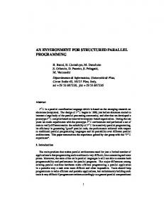
pRPL was written in C++ and built upon the Message Passing Interface (MPI), which is a de facto standard parallel programming library composed of a set of functions that enable and manage parallel computing by passing messages between processors [1]. Since MPI and C++ compilers are available on almost all parallel computing systems (e.g., massive parallel computers, and computer clusters), the portability of pRPL is guaranteed, and the applications built upon it will be portable across different parallel computing platforms as well. From a software architecture perspective, pRPL serves as a middleware connecting the general-purpose parallel programming library (i.e., MPI) and the application-specific raster-processing programs. It hides the complex technical details of parallel computing from the users, thus relieves them from the time-consuming parallel programming and lets them only focus on the algorithms themselves. Mineter and Dowers [2] referred to this kind of architecture as a layered approach to parallel processing for geographic applications (Figure 1).
Categories and Subject Descriptors
D.1.3 [Software, Programming Techniques]: Concurrent Programming – Parallel programming.
General Terms Performance
Keywords
Parallel, raster, programming library
1. INTRODUCTION TO pRPL
From a parallel computing perspective, raster is born to be parallelized. A raster dataset is essentially a matrix of values, each of which represents the attribute of the corresponding cell of the field (e.g. land use type, elevation, etc). A matrix can be easily partitioned into sub-matrices and assigned onto multiple processors so that the sub-matrices can be processed simultaneously and a higher processing speed will be reached.
Figure 1 pRPL in a layered architeture
pRPL was developed by the author to encapsulate complex parallel computing utilities and routines specifically for raster processing (e.g., raster data decomposition, distribution and gathering among multiple processors, inter-processor communication and data exchange), and provide an easy-to-use interface for users to parallelize almost any raster-processing algorithm with any arbitrary neighborhood configuration. pRPL greatly reduces the development complexity. Moreover, even though pRPL was developed for massive-volume geographic raster processing, it can also be used for other large-scale rasterlike computations such as image processing and Cellular
2. FEATURES OF pRPL 2.1 OOP library and class templates
pRPL is an Object-Oriented programming library, and provides a set of classes 1 for users as the interface to easily manage and control the underlying parallel processes. Also, pRPL is a template programming library, and supports any type of cell attribute values, e.g. integer numbers, single and double precision floating point numbers, and even more complex user-defined data structures.
1
The SIGSPATIAL Special, Volume 1, Number 1, March 2009 Copyright is held by the author/owner(s).
57
For more technical details of pRPL, see the user manual Getting Started with pRPL [13]
the cellspace by rows, or columns, or blocks, without considering the workloads associated with the cells, and produces equal-area sub-cellspaces. Irregular decomposition, on the other hand, takes account for the workloads of the cells, and is likely to produce unequal-area sub-cellspaces in order to divide the workloads more evenly among the sub-cellspaces. pRPL provides a quad-treebased (QTB) decomposition method. The QTB decomposition is an iterative process. At each iteration, the workloads associated with the leaves (i.e., sub-cellspaces) are calculated, and the leaf with the largest workload will be divided into 4 child leaves. The quad-tree will keep growing until the maximum number of leaves or the minimum workload associated with a sub-cellspace is reached. Caution must be taken when this decomposition method is to be used, because the extra computation required to construct the quad-tree and to calculate the workloads of the sub-cellspaces might outweigh the speed-up gained from the better workload distribution.
2.2 General support for raster processing
As a general-purpose library, pRPL was developed to parallelize most raster-processing algorithms as long as the transition computation is parallelizable, i.e., the computation for a certain cell (or pixel) within the output cellspace is independent of that for other cells. Thus, neighborhood-scope (or moving-windowbased) and local-scope (which can be seen as special cases of neighborhood-scope ones) algorithms are fully supported by pRPL, and some regional-scope and global-scope algorithms that meet the parallelizability criterion are also supported. pRPL supports any arbitrary neighborhood configuration (Figure 2). The neighborhood can be either continuous or discontinuous (Figure 2d), either symmetrical or asymmetrical (Figure 2e). Furthermore, the cells within a neighborhood can be assigned with different weights for kernel-based local processing [3].
Figure 4 Domain decomposition methods in pRPL Figure 2 Examples of neighborhood configuration
2.5 “Update-on-Change” and the Valueheaded index stream for data exchange
Also, the transition algorithm to be parallelized can be either centralized or non-centralized. A centralized algorithm only evaluates and updates the central cell of the neighborhood, whereas a non-centralized algorithm may evaluate and update any cell(s) within the neighborhood. A finalizing process can be included in the algorithm, e.g., assigning a value to the cell based on an intermediate value of the cell calculated during the evaluation process.
When a neighborhood-scope algorithm is used, the transition computation for a certain cell requires the values of its neighboring cells. In consequence, a sub-cellspace has to include not only the block of cells to be processed, but also a “halo” of cells surrounding the block [4], which can be seen as the replicas of the cells within the neighboring sub-cellspaces. The “halos” of the sub-cellspaces must be updated after each iteration, if an iterative algorithm is used. When the origins are updated, the replicas should be updated accordingly. This inevitably creates the communication overhead (i.e., messages in the MPI environment) between processors. However, not all the “halo” cells’ values are changed after a certain iteration, and it would be inefficient to refresh all the “halo” cells each time. pRPL uses a mechanism called “Update-on-Change”, and only updates the halo cells whose origins have been changed at an iteration, which significantly reduces the volume of the messages passed among processors. Also, the messages are constructed in value-headed global-index streams instead of arrays of coordinate-value pairs. A value-headed global-index stream contains the information of the “halo” cells to be updated within the sub-cellspace. It starts with an attribute value (any type) and an integer number
2.3 Multi-layer processing
Multi-layer processing is commonly used in raster-based GIS and GeoComputation algorithms, as well as in other kinds of image processing, e.g., an AND operation on two binary-coded images. pRPL supports multi-layer algorithms by allowing users to associate multiple Layer objects to a Transition object which implements the raster-processing algorithm. Each Layer object can contain a cellspace (CellSpace object), and/or multiple subcellspaces (SubSpace objects), and a Neighborhood object (Figure 3).
2.4 Regular and irregular decomposition
pRPL provides both regular and irregular decomposition methods to divide the domain (Figure 4). Regular decomposition divides
58
processors continue working on the interiors of the sub-cellspaces, and then finally complete the communications. The “edgesFirst” provides a means to improve the performance by overlapping communication and computation.
indicating the number of indices following this attribute value, followed by a string of global indices of the cells that are to be updated to this value; then another attribute value and an integer number, and a string of indices of cells updated to the second value; and so on so forth (Figure 5b). The indices are determined in the global spatial extent, and can be easily translated into/from local coordinates within sub-cellspaces. The value-headed globalindex stream is usually more efficient than an array of coordinatevalue pairs (Figure 5a) in terms of message volume. In many cases, there are only a limited number of attribute values that can be assigned to a cell, and many cells will be updated to the same values, thus there is no need to include every cell’s value in the messages. For example, if there are M integer values that the “halo” cells will be updated to, and N “halo” cells to be updated, then (2M+N)×sizeof(integer) bytes are needed for this message when the value-headed index stream is used, but 3×N×sizeof(integer) bytes are needed when the coordinate-value pairs are used. Apparently, when M is small and N is big, the value-headed global-index stream will be much smaller than the array of coordinate-value pairs.
Figure 6 The structure of a 10×10 sub-cellspace with a 3×3 neighborhood
2.7 Processor grouping, data-parallelism and task-parallelism
pRPL organizes processors in groups. The initial set of processors (i.e., all the engaged processors) constitute the root group. The root group can be divided into sub-groups, which can be further divided into smaller groups. Each group has a master. Groups of processors can be assigned with different datasets and transition processes. Thus pRPL supports both data-parallelism and taskparallelism. When a dataset is divided and distributed among the processors within a group, or among the groups, data-parallelism takes place. When different transition processes are assigned to multiple groups, task-parallelism among groups takes place (within groups, data-parallelism takes place because the dataset will be divided and distributed among the processors).
Figure 5 Coordinate-value pairs (a) and Value-headed globalindex stream (b)
2.6 Non-blocking communication and “edgesFirst” for data exchange
2.8 Static and dynamic load-balancing
When a transition process (i.e., the raster-processing algorithm) is to be applied on a sub-cellspace, the sub-cellspace’s “halos”, edges and interior (Figure 6) will be automatically determined by pRPL according to the transition‘s characteristics, the neighborhood’s configuration, and the sub-cellspace’s location within the global spatial extent. Halos, as mentioned before, are the replicas of the cells within the neighboring sub-cellspaces, whereas edges are the origins of the “halo” cells in the neighboring sub-cellspaces. The interior is the rest of the subcellspace. When data exchange is needed, e.g., after an iteration of an iterative algorithm, the changed edge cells will be compressed into value-headed global-index streams and sent to the neighboring sub-cellspaces, and also streams from the neighboring sub-cellspaces will be received and the “halo” cells whose origins have been changed will be updated accordingly. Instead of blocking communication, pRPL uses non-blocking communication routines, which allows message passing while the processors are working on other tasks (e.g. computation, I/O process), whereas blocking communication forces the processors to wait until the communication is completed [5]. pRPL provides an “edgesFirst” option for users, which forces the processors to first process the sub-cellspace’ edges, then start exchanging the “halo” information. During the data-exchange communication, the
After a dataset is divided and distributed among the processors within a group, the sub-cellspaces are statically assigned onto the processors, and will not be re-allocated among the processors once the computation starts, because moving the sub-cellspaces among processors’ local memories could cause extreme communication overheads, given that the sizes of the subcellspaces are usually large. This load-balancing mechanism is referred to as static load-balancing. However, in some cases, e.g., calibrating the transition parameters of a model, the same dataset will be assigned to a set of processor groups, and a “task farm” can be used to assign different tasks (e.g., transition parameters) to the groups in respond to their requests. Thus, a dynamic loadbalancing mechanism can be implemented among the groups. In one word, pRPL supports both static and dynamic load-balancing.
3. COMPARING pRPL WITH OTHER SIMILAR PROGRAMMING LIBRARIES
Several other parallel raster-processing programming libraries similar to pRPL have existed. The Global Arrays (GA) toolkit, developed by the Pacific Northwest National Laboratory, provides a shared memory style programming environment in the context of distributed array data structures for users to manipulate
59
developed at the University of California, Santa Barbara, to simulate and forecast the spread of urbanization across the landscape over time [8-10], and its name comes from the GIS layers incorporated into the model: Slope, Landuse, Exclusion (where growth can not occur, e.g., oceans, parks), Urban, Transportation, and Hillshade [11].
2D arrays [6]. The Parallel Utilities (PUL), developed by the Edinburgh Parallel Computing Centre at the University of Edinburgh, was developed on top of MPI and provides a suit of utilities to parallelize algorithms. PUL has been used to implement several fundamental GIS operations, i.e., vector-toraster conversion, raster-to-vector conversion, and vector polygon overlay, and some GIS applications, e.g., raster generalization [7].
The basic unit of a SLEUTH simulation is a growth cycle, which usually represents a year of urban growth. A simulation (or a Run) consists of a series of growth cycles that begins in the start year and completes in the stop year. Four growth rules are applied on the space during each growth cycle: Spontaneous growth rule, New Spreading Centers rule, Edge growth rule, and RoadInfluenced growth rule. Five parameters (or coefficients) are included in SLEUTH: Dispersion, Breed, Spread, Slope, and Road Gravity. Their values range from 0 to 100, and determine how the growth rules are applied. Also, a self-modification process is embedded at the end of each growth cycle to modify the parameter values according to the growth rate.
The major differences between pRPL and these two parallel programming libraries are the following. 1. GA and PUL were developed for experienced programmers who wish to fully utilize the parallel computing systems and develop portable high-performance programs without spending too much time dealing with the underlying details. They are both written in Fortran and C, and procedural-based programming libraries. Users write GA-based and PUL-based programs by calling the functions defined in the libraries. GA and PUL provide many low-level functions for users to explicitly control the processing, e.g., data exchange between data blocks, but lack of high-level functions for easy programming (even though PUL provides the skeleton interface which contains some high-level functions).
Calibration processes are needed to determine the appropriate parameter values so that SLEUTH can produce more realistic simulation results. The basic calibration procedure of SLEUTH is to compare multiple testing results produced using a set of parameter combinations with the goal dataset(s) that usually are real historical geospatial data in order to determine the best-fit parameter combination(s). In addition, to simulate the random processes that happen during the urban growth, the Monte Carlo method is used. For a single parameter combination, a simulation may be executed multiple times with different Monte Carlo seed values. In practice, 10~100 Monte Carlo iterations for each parameter combination are suggested.
In contrast, pRPL was developed primarily for the general geographers (and other geospatial professionals) who wish to speed up their raster-based processing and shorten the waiting time but do not have much parallel programming experience. Thus the simplicity of usage was given higher priority than performance. It is written purely in C++, and is an object-oriented library. A collection of C++ classes are provided as the interface and hide the parallel processing details from users. Objectoriented programming has the advantage over procedural-based programming for its intuitiveness in the system design and implementation processes.
The complex transition rules, the multiple parameters, the Monte Carlo method, and the potential vast volume of the datasets, make the calibration of SLEUTH extremely computationally intensive. “The model calibration for a medium sized data set and minimal data layers requires about 1200 CPU hours on a typical workstation” [12].
The classes in pRPL provide high-level methods that combine other low-level methods to perform some complicated processes. For example, calling only one method of the Layer class, e.g., smplDcmpDstrbt(), performs the decomposition of the global cellspace on the master processor and the distribution of the subcellspaces to other processors. Then calling another method of the Layer class, i.e., update(), applies the user-defined transition on the sub-cellspaces, and pRPL automatically handles the necessary data exchange without any other extra work from the user.
In this study, pSLEUTH3, the parallel version of SLEUTH, was developed to improve the computational performance of the SLEUTH model, especially the calibration processes, by fully utilizing the advanced features of pRPL. The four growth rules of the SLEUTH model were implemented using pRPL, thus the data layers used in the model will be decomposed and distributed onto multiple processors. Table 1 shows the centralization and scope characteristics of the growth rules. The Transition classes that implement the growth rules were developed according to these characteristics. For example, the Road-Influenced growth rule involves a random walk along the road network, thus the whole road cellspace is required by this rule which makes it a globalscope transition. In consequence, unlike other data layers, the whole road cellspace has to be broadcasted to all the processor (cellspace2 in Figure 3).
2. pRPL recognizes the spatial distribution of workload over the space and provides the workload-sensitive QTB decomposition method, i.e., the quadDcmp() method of the Layer class, to divide the datasets in a better balanced way. Both GA and PUL provide regular decomposition methods, but do not have any function to directly produce irregular decomposition. In order to perform a workload-based decomposition, users of GA and PUL have to write their own functions which can be quite complex.
4. EXPERIMENTS AND PERFORMANCE 4.1 Introduction to pSLEUTH
To evaluate the performance of pRPL, the well-known urban land-use change model, SLEUTH2, was parallelized using pRPL. The SLEUTH model is a Cellular Automat (CA) model 2
Growth Rule
Centralization Type
Scope Type
Spontaneous
Centralized
Neighborhood-scope
3
For more information about SLEUTH, see the website of Project Gigalopolis: http://www.ncgia.ucsb.edu/projects/gig/
60
For more information about pSLEUTH, see the user manual – Getting started with pSLEUTH [14]
New Spreading Centers
Non-Centralized
Neighborhood-scope
Edge
Non-Centralized
Neighborhood-scope
Road-Influenced
Non-Centralized
Global-scope
Table 1 Characteristics of the growth rules of SLEUTH With pRPL, pSLEUTH organizes the processors in groups, and assigns each group a subset of the parameter combinations to be evaluated. Within a group, the data layers are divided and distributed among the processors. In this way, the data-task hybrid parallelism is realized. In addition, pSLEUTH provides two options of load-balancing for the task parallelism among the processor groups: static tasking and dynamic tasking. When static tasking is used, the subsets of the simulations (i.e., parameter combinations) are assigned to the groups before the actual computation starts. When dynamic tasking (Figure 7) is used, a master-worker organization will form, which consists of a master processor (or the emitter processor), and a set of worker-processor groups. Each worker group will be initially assigned with a subset of simulations, and a task farm that contains the remaining simulations will be created on the emitter processor. When a group finishes its initial set of simulations, it requests for a new task, i.e., a simulation, from the task farm. The emitter processor keeps sending tasks to the worker groups until the task farm is drained.
Figure 8 The 1980 urban areas (in blue) and the simulated 1980-1990 expansions (in red)
5. CONCLUSIONS
pRPL can be used to parallelize almost any raster processing algorithm with any arbitrary neighborhood configuration. pRPL supports multi-layer algorithms and provides different datadecomposition methods for users. Especially, a spatial-adaptive decomposition method (i.e., the QTB decomposition) is provided for the cases when the computational intensity is extremely heterogeneous over the space. The “Update-on-Change” and Value-headed global-index stream techniques help reduce the communication overhead for data exchange among the processors, hence reduce the computing time. Furthermore, the “edgesFirst” and non-blocking communication techniques overlap the computation and communication, which also helps reduce the computing time. pRPL organizes processors in groups, and supports both data-parallelism and task-parallelism. With grouped processors, dynamic load-balancing can be implemented with ease. Experiments with real-world datasets shows that pRPL yields satisfyingly high speed-ups and efficiencies. In conclusion, as a generic parallel library, pRPL effectively reduces the development complexity of parallel programming, and efficiently reduces the computing time.
Figure 7 Dynamic tasking for pSLEUTH
4.2 Experiments and performances
6. REFERENCES
A dataset of the continental US urban areas (4948×3108) was used to conduct a series of experiments (Figure 8). A calibration scenario was specified as follows: only two historical urban area data (1980 and 1990) are used, only three values (0, 50, 100) will be evaluated for each parameter, and only 1 Monte Carlo iteration will be performed. Thus the total number of simulations is 243 (= 35), and each simulation includes 11 ( = 1990-1980+1) years. The experiments were conducted on a Dell cluster which is composed of a Dell 1750 dual CPU 3.06GHz Xeon servers and a single Dell 1750 monitoring node. The head node has 4GB RAM, 2 mirrored system disks, and a 2TB RAID array that is shared to the cluster. The 128 compute nodes have 2GB RAM each.
[1] W. Gropp et al., MPI: The Complete Reference (Vol. 2), Cambridge, MA, USA: The MIT Press, 1998. [2] M.J. Mineter and S. Dowers, “Parallel Processing for Geographical Applications: A layered Approach,” Journal of Geographical Systems, vol. 1, 1999, pp. 61-74. [3] C.D. Lloyd, Local Models for Spatial Analysis, Boca Raton, FL, USA: CRC Press, 2007. [4] M.J. Mineter, “Partitioning Raster Data,” Parallel Processing Algorithms for GIS, Bristol, PA, USA: Taylor & Francis, 1998, pp. 215 - 230. [5] M. Cosnard and D. Trystram, Parallel Algorithms and Architecture, Boston, MA: International Thomson Computer Press, 1995.
When 32 processors were divided into 8 groups with dynamic tasking, the column-wise decomposition was used, and each processor held 8 sub-cellspaces, the speed-up reached 24 (Figure 9). Note that when dynamic tasking is used, the emitter processor does not participate in the computation. In Figure 9, for dynamic tasking experiments, the number of processors does not include the emitter processor.
[6] J. Nieplocha et al., “Global Arrays User Manual,” 2007; http://www.emsl.pnl.gov/docs/global/um/GA.pdf.
61
[11] N.C. Goldstein, J.T. Candau, and K. Clarke, “Approaches to Simulating the "March of Bricks and Mortar",” Computers, Environment and Urban Systems, 2004, pp. 125-147.
[7] R. Healey et al., Parallel Processing Algorithms for GIS, Bristol, PA: Taylor & Francis, 1998. [8] K.C. Clarke, S. Hoppen, and L. Gaydos, “A Self-modifying Cellular Automaton Model of Historical Urbanization in the San Francisco Bay Area,” Environment and Planning B: Planning and Design, vol. 24, 1997, pp. 247-261.
[12] K.C. Clarke, “Geocomputation's Future at the Extremes: High Performance Computing and Nanoclients,” Parallel Computing, vol. 29, 2003, pp. 1281-1295. [13] Q. Guan, “Getting started with pRPL,” 2008; http://www.geog.ucsb.edu/~guan/pRPL/Getting_started_w ith_pRPL.pdf.
[9] K.C. Clarke and L.J. Gaydos, “Loose-coupling a Cellular Automaton Model and GIS: Long-term Urban Growth Prediction for San Francisco and Washington/Baltimore,” International Journal of Geographical Information Science, vol. 12, 1998, pp. 699-714.
[14] Q. Guan, “Getting started with pSLEUTH,” 2008; http://www.geog.ucsb.edu/~guan/pRPL/Getting_started_w ith_pSLEUTH.pdf.
[10] E.A. Silva and K.C. Clarke, “Calibration of the SLEUTH Urban Growth Model for Lisbon and Porto,” Computers, Environment and Urban Systems, vol. 26, 2002, pp. 525– 552.
Figure 3 Multiple layers can be used in pRPL
Efficiencies of static and dynamic tasking with column-wise decomposition
Speed-ups for static and dynamic tasking with column-wise decomposition
1.2
25
1
Speed-up
20
Static Dynamic - 2 groups
15
Dynamic - 4 groups Dynamic - 8 groups
10
Efficiency
30
0.8
Static Dynamic - 2 groups
0.6
Dynamic - 4 groups Dynamic - 8 groups
0.4 0.2
5
0
0 1
2
4
8
16
1
32
2
4
8
16
32
Number of processors
Number of processors
Figure 9 Performances for static and dynamic tasking with columnwise decomposition (each processor holds 8 sub-cellspaces)
62