Pruning and Regularization Techniques for Feed Forward Nets applied on a Real World Data Base Matthias Rychetsky, Stefan Ortmann, Manfred Glesner Darmstadt University of Technology Institute for Microelectronic Systems Karlstraße 15, D-64283 Darmstadt, Germany E-Mail:
[email protected] Key-words: weight pruning, regularization, neural network optimization, knock detection Abstract - In this paper we present an extensive study of weight pruning and regularization techniques for feed forward neural nets. This algorithm comparison is based on a data base of known benchmark data sets and a realistic real world data set from automotive control. We trained 30 nets for every algorithm implemented by us, with three different ways of data set splitting. For the 38 implemented methods this results into totally 1140 trained nets.
1 Introduction In order to construct a network with the best generalization performance (no overfitting or underfitting) it is desirable to construct a neural net with just the right size for a given problem. Other reasons for network optimization are computational and storage costs of the trained net and speed up of the learning process. This optimal size can be achieved through constructive learning algorithms which grow a network appropriate for the data, or by removing parts of the net. This latter process is called pruning (see [2] for an overview). Furthermore pruning
techniques can be used to avoid overfitting to the data and therefore they could be interpreted as regularization techniques. There exist many methods for neural network regularization, which can be mainly divided into three categories: Techniques based on cost terms, overfitting avoidance through training control, and some other techniques like weight sharing. Through pruning one can remove two possible elements in a neural network: Neurons and weights. Neuron pruning has advantages especially in the perspective of hardware implementation, due to the fact that by the removal of neurons the network calculation can be simplified significantly. In [1] we presented a comparison between three new correlation based neuron pruning algorithms and known techniques applied to the same data base used here. These statistical approaches can significantly reduce multi-layer perceptron network size and improve network performance in the sense of generalization error. They use the correlation between the neuron output and the network error (NONECS = neuron output network error correlation saliency), a correlation between the error at a neuron and net error (NENECS = neuron error network error correlation saliency) an d finally a regression analysis of the last correlation (NENEPS = neuron error network polynomial saliency)
N e u r a l n e tw o r k o p tim iz a tio n te c h n iq u e s G r o w in g te c h n iq u e s
P r u n in g te c h n iq u e s
N e u r o n P r u n in g
W e ig h t P r u n in g
S a lie n c ie s M a g n itu d e b a s e d R e le v a n z m e a s u r e o f K a r n in R e le v a n z m e a s u r e o f F in o ff O p tim a lB r a in D a m a g e B F O R C E O p tim a lB r a in S u rg e o n
P r u n in g m e th o d s ta tic
S a lie n c ie s
P r u n in g m e th o d
S k e le to n iz a tio n
N e u r o n S im p le P r u n e
D y n a m ic M ix tu r e o f E x p e rts C a s c a d e C o r r e la tio n
R e g u la r iz a tio n te c h n iq u e s
C o s t te rm s W e ig h t D e c a y (W e rb o s )
C o n s tr u c tiv e S u b -F e a tu re D e te c to r N e t
W e ig h tE lim in a tio n ( C h a u v in )
W e ig h tS im p le P r u n e
N O N E C S
N e tw o rk B o o s tin g
W e ig h tD e c a y (Is h a k a w a )
A u to P ru n e
N E N E C S
B a g g in g
W e ig h tD e c a y ( C h a u v in )
N E N E P S
D y n a m ic N o d e C r e a tio n ( D N C )
W e ig h tE lim in a tio n ( W e ig e n d )
d y n a m ic L a m b d a P ru n e
B F O R C E
E p s iP r u n e
IM - S k e le to n iz a tio n
R e s o u r c e A llo c a tio n N e tw o rk s (R A N ) P r o je c tio n P u r s u it R e g r e s s io n ( P P R )
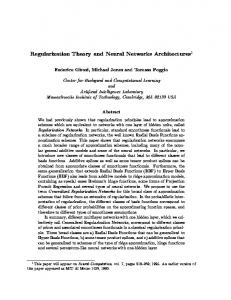
FIGURE 1. Neural network optimization techniques overview
O v e r fittin g a v o id e n c e E a r ly S to p p in g E x te n d e d E a r ly S to p p in g
im p le m e n te d
O th e r te c h n iq u e s S o ftW e ig h tS h a r in g L o c a l B o ttle n e c k s D is tr ib u te d B o ttle n e c k s
n o t im p le m e n te d
Neuron pruning is very sensitive, therefore only one neuron at a time can be removed. On the other hand weight pruning is finer in its results and it is usually easy to remove a large amount of network weights. Weight pruning techniques can be used to find just the right network size and to improve network performance. To approach the pruning problem the following tasks have to be solved:
size). Due to the fact that after a small increase of Ev the error often comes down again, Lutz Prechelt defined a condition which allows small error increases during the training process [6]. Using the generalization loss GL (increase of the current validation error Ev against the best validation error in the whole learning process Ev,opt): Ev ( t ) GL ( t ) = 100 --------------------- – 1 Ev, opt ( t )
1. “Pruning time” or “when should be pruned” 2. “Pruning strength” or “how many elements should be removed” 3. “Saliency” or “which elements should be pruned” 4. “Pruning stop condition” or “when should the pruning process end” The best method to remove weights is that one that uses the exact increase in the network error as a measure if the weight is removed (see below). Since it is computationally expensive to calculate for all possible weights (and combinations of weights) this increase, a measurement of relevance system has to be developed which approximates it. This sensitivity measure or saliency will be discussed in the next section. In this paper we are focusing only on methods for Multi-Layer-Perceptron nets. For other network types similar techniques are available. Figure 1 shows a taxonomy of neural network optimization techniques (this claims not to be complete). The field of neural network optimization can be partioned into three fields: Growing, pruning and regularization techniques. The first and very interesting topic will be not treated here (examples can be found in [12][13]). Some regularization techniques are discussed in the next section. In section 3 and 4 weight pruning methods are discussed (neuron pruning methods can be found e.g. in [1] and [2]). Section 5 shows the results of this study for our data base.
2 Regularization techniques In this section we briefly review the regularization techniques used in this study. We are using here regularization methods from two fields: Overfitting avoidance by learning control and complexity bounding by cost terms. For first case we examined Early Stopping and Extended Early Stopping. They are both based on an error increase of the validation error. The Early Stopping condition is: UP = [ E v ( t ) > E v ( t – k ) ] ∧ [ E v ( t – k ) > E v ( t – 2k ) ] (Eq. 1)
The condition UP is true, if the sum squared validation error Ev increases in two intervals (k is the training strip
(Eq. 2)
the training is stopped if a threshold for GL is exceeded. Figure 2 shows a typical training using both stopping conditions. To get the best net for Extended Early Stopping the network parameters are saved every time a new Ev,opt is reached. After the training stop (here Z2) the parameters of point Z1 corresponding to Ev,opt are restored. 2
1 0
E a r ly s to p p in g
V a lid a tio n e rro r
1
1 0
E x te n d e d E a r ly S to p p in g
1 0
0
0
5 0
1 0 0
1 5 0
2 0 0
2 5 0
E p o c h s
Z 1
Z 2 3 0 0
3 5 0
4 0 0
FIGURE 2. Early and Extended Early Stopping Cost term based regularization is represented in this study by Weight Decay (after Werbos [9]) and Weight Elimination (from Chauvin [8]). Using an additional cost term in the error function, unimportant weights are pushed towards zero. Weight Decay uses here the cost term 1 C = --- λ ∑ w i2 2
(Eq. 3)
i
Weight Elimination has generally the cost term wi2 ⁄ w 02 1 C = --- λ ∑ -------------------------2 1 + w2 ⁄ w2 i
i
(Eq. 4)
0
By choosing w0 one can influence the weight magnitude distribution: Large values of w0 lead to nets with many small weights and small values of w0 lead to nets with few big weights. With w0=1 we have chosen a small
value to get many weights which are nearly zero (like Chauvin in [8]). These two techniques are especially useful together with magnitude based weight pruning methods and can improve their performance significantly.
3 Saliency as a measure of relevance Basis of the saliency definition as a measure of relevance is the increase in the net squared error if one weight is removed and the rest of the net remains unchanged: ρ i = E without weight i – E with weight i
(Eq. 5)
Instead of calculating this relevance measure for every weight directly, pruning strategies try to approximate it for each unit. In this section methods are described to do this estimation and for comparison the first order brute force solution is defined.
3.1 Magnitude Based Pruning The simplest method for calculating the importance of a weight is used in magnitude based pruning. It assumes that the weight with the smallest value has the smallest contribution to the performance of the net. This pruning method removes only the smallest weights from the net.
(OBD) by Le Cun, Denker and Sara [7]. OBD uses an approximation to the second derivative of the error with respect to each weight to determine the saliency of the removal of that weight (this avoids the calculation of the full Hesse-matrix). Optimal Brain Surgeon (OBS) is a more accurate method which avoids the approximation. But it is computationally very expensive, because it has a complexity of O(n2) if the net has n weights for every pruning step to determine the saliencies. Therefore we only included OBD in this study (the pruning improvement justifies in no way the additional computing overhead).
3.4 Brute Force The above described saliencies calculate the relevance of weights by an estimation of the error increase when weights are removed. To compare this we also computed for the experiments the exact increase of the error through weight removal. If this is done for every weight in the net, the best choice can be made and the weights with the smallest impact on the net error can be removed. This is a first order optimal strategy in the sense that it only selects the best weights to prune based on the method described above. It neglects the fact that it could matter in which order the weights are removed (high order correlation).
4 Pruning algorithms 3.2 Karnin’s and Finnoff’s saliency A second relatively simple saliency was developed by Karnin [10]. He estimated the sensitivity of the network error to the removal of weights during learning process. To do this the following equation is used: f
0
E ( wij ) – E ( wij ) f - w ij S ij = – ----------------------------------------f 0 w ij – w ij
(Eq. 6)
where wfij is the value of the weight ij at the end of the training and w0ij is an idealized initial state, where all weights have the value 0. To calculate the above defined saliency many approximations are made, e.g. the initial state is approximated by small random weight values and the error is taken at this real initial state. Finnoff defined a statistical significance test, which calculates the significance of weight deviations from zero during the learning process [5].
3.3 Optimal Brain Damage A method which does a mathematical approximation of the relevance of a weight is Optimal Brain Damage
4.1 Weight Simple Prune After the calculation of a relevance measure it is necessary to define an algorithm which can prune the weights automatically. While the saliency gives the possibility to select prunable weights, the pruning algorithm has to determine the pruning time and the end of the pruning process. Normally in the literature simple assumptions about the pruning process are made (e.g. [7]). Based on this assumptions an informal description of pruning is done. To formalize our study we defined a simple pruning algorithm (called Weight Simple Prune). TABLE 1. Pre training stopping conditions Criterion
Condition
Defaults
Extended Early Stopping
GL>GLmax
GLmax=5..10%
Maximal number of epochs
ne>ne,max
ne,max=1000..500 0
Minimal number of epochs
ne>ne,min
ne,min=50..100
After a pre training of the net, which is executed until the stopping conditions of table 1 , we applied a main training phase where several times a pruning step is involved. This main training phase is stopped if a given percentage ωpr of the weights have been removed, the generalization loss GL (increase of validation error against the best achieved error) is above a threshold GL max or a predefined number of epochs ne is exceeded. Using the number of removed weights npr and the initial weights number nw the removed percentage is defined by: n pr ω pr = ------- ⋅ 100% nw
(Eq. 7)
Weight Simple Prune is a static technique that always removes a fixed percentage of weights (of the initial count) in every pruning step. As a rule of thumb one can apply about 5% for this pruning strength (in small nets this can be reduced to 1%). The pruning is started every time if overfitting appears or, in the cases without overfitting, if the change in the training error is very small (e.g. ωpr,max
ωpr,max=90..95%
Maximal number of epochs
ne>ne,max
ne,max=5000
The parameters λmax (maximum of pruning threshold) and α have to be chosen appropriate. GL is the loss of generalization performance at the pruning point. It should be mentioned that Lambda Prune needs a certain generalization loss for correct pruning.
Maximal generalization loss
GL>GLmax
GLmax=100%
4.4 Epsi Prune
4.2 Auto Prune AutoPrune, developed by Finoff, Hergert and Zimmermann [5], is very similar to Weight Simple Prune but it has two main differences:
The second techniques specialized on Finnoffs saliency is Epsi Prune. Here simply a threshold ε > 0 is used for pruning. All weights with a saliency smaller then ε are removed. After a pruning step the threshold is incremented by ∆ε until a maximum value is reached. In the first pruning step ε is set to: εinit=MIN(Saliencies).
1. The pruning strength is decreased after the first pruning step and stays at fixed value to the end of the pruning process. This behavior was chosen by the developers because in the case of big nets a removal of a large amount at the beginning improves results.
A nice property of Epsi Prune is that it can also be used to calculate the saliency for weights which have been already removed from the net. Therefore removed weights could be reactivated.
2. Normal you take a higher value for the pruning strength. This improves the pruning speed, but the risk to miss the “right” network size has to be taken into account.
5 Experiments
For problems where massive overfitting occurs, Auto Prune can outperform Weight Simple Prune because it can avoid the overfitting through a fast removal of use-
In the following section we describe the carried out experiments and compare the results with respect to computational complexity, impact on generalization performance measured through test set error and classification rates and finally to network complexity.
The presented five techniques as well as normal training without pruning were applied to standard data sets (IRIS, GLASS) and some realistic data from combustion engine control (FILU data). The IRIS problem is a simple classification task in which the network has to determine the correct biological subclass for iris flowers. The GLASS problem is a more complicated task, in which the network has to classify glass types using chemical components and the refraction index of small glass splinters. In the engine control task knocking has to be detected, a process which could damage the engine and therefore has to be avoided (for more details see [11]). This task was split into two subtasks for different engine speeds, the first data set containing data measured at 2000rpm (FILU2000) and the second containing data measured at 4000rpm (FILU4000). Due to the noise introduced by the large amount of vibration in the engine at 4000rpm the second data set was the hardest classification task for the network.
v ,ttc
0 ,8
E
IR IS
E
v ,p ru n e v ,ttc
G L A S S F IL U 2 0 0 0 F IL U 4 0 0 0
0 ,6
0 ,4
F IL U 2 0 0 0
D e = 1 .0
D e = 0 .1
D e = 0 .5
l= 1 .0
E p s iP r u n e
l= 0 .8 5
l= 0 .6 6 6
O B D
M B P
B F o rc e
F in n o ff
K a r n in
O B D
B F o rc e
K a r n in
F in n o ff
L a m b d a P ru n e
G L A S S
0 ,6
A u to P ru n e 1 5 -5
IR IS
M B P W E *
M B P
M B P W D *
W e ig h tS im p le P r u n e
0 ,8
E
1
0
1
v ,re g
1 ,2
0 ,2
1 ,2
E
simple benchmark data sets. The FILU data is only classified with a 3% better sum squared error. But this is mainly caused by the very well classification performance on these problems (FILU2000 about 1% of missclassified patterns; FILU4000 about 5-6% of missclassified patterns). The results of the early stopping techniques justify their standard application in the first training phase (especially if Extended Early Stopping is used)
F IL U 4 0 0 0
0 ,4 0 ,2 0
FIGURE 3. Comparison of validation errors using regularization (Ev,reg) against the error with training to convergence (Ev,ttc) Using this data base we first started with a normal training procedure (train to convergence of test set error). Then we applied the regularization techniques Early stopping and Extended Early Stopping, Weight Decay and Weight Elimination. The two Early Stopping methods are not used for FILU data, because this data shows nearly no overfitting (this is due to the fact that the database contains that much data, that training and validation set are statistically very similar). Weight Decay and Weight Elimination were tested with different regularization parameters λ. Figure 33 shows the performance comparison based on the ratio of the (sum squared) validation error using regularization Ev,reg to the validation error Ev,ttc using train to convergence. Values smaller than one indicate an improvement through regularization. As you can see regularization (especially the simple weight decay) is able to reduce the validation error up to 28%. But this big improvement is only achieved for the
FIGURE 4. Comparison of validation errors using pruning (Ev,prune) against the error with training to convergence without pruning (Ev,ttc) In the next series of experiments we trained and pruned multi-layer perceptron nets using the four pruning methods presented above (Weight Simple Prune, Auto Prune, Lambda Prune, and Epsi Prune). For Weight Simple Prune and Auto Prune all saliencies where applied. In the case of Weight Simple Prune with the saliency Magnitude Based Pruning (MBP) the regularization techniques Weight Decay and Weight Elimination are applied additionally (here λ is select from the best results of the first experiment using only regularization). Due to the fact that Lambda- and Epsi Prune are specialized on the saliency of Finnoff the two algorithms where used only with this saliency. For all trials the mean values of removed weights, maximum value of removed weights, error on training set, validation error, epochs needed and the computational costs (measured in flops) were recorded (please contact the authors for the full data base). In Table 3 two representative groups of pruning results (percentage of pruned weights) are shown. The results were chosen after two different optimization criteria: In the first case the net was selected which has the lowest sum squared error on the validation set. The second criterion selects the smallest resulting net.
6 Conclusion In this paper we presented a study of neural network pruning and regularization techniques. They have been tested in a systematic way on a large real world data base. In order to present statistically significant results for every algorithm 3 times 30 networks have been calculated. Comparing the pruning strategies one must at first notice that the pruning results (decrease of validation error, pruned weights etc.) strongly depend on the data set and its complexity. Nevertheless some general conclusion can be drawn: If you want to construct the smallest possible network, one should choose as pruning algorithm Weight Simple Prune or Auto Prune. As saliencies in both cases Magnitude Based Pruning (especially in connection with Weight Elimination) and the straight for-
ward Brute Force show good results (also Karnin’s saliency). Optimal Brain Damage and the saliency of Finnoff and also Lambda and Epsi Prune can not reach this performance for weight removal. If weight pruning is used to improve the generalization performance Epsi Prune should be used (also Weight Simple Prune and Auto Prune using Brute Force and Karnin’s saliency perform well). For this optimization goal also regularization techniques are well suited (e.g. Weight Decay; Early Stopping should be used in all applicable cases). The computational costs (FLOPS) of all algorithms differ only by a factor of about 5. If the problem is simple or the starting net is largely oversized the computational costs compared to training to convergence are reduced. In other cases the maximum observed increase was 4.9 (using Epsi Prune). Even Brute Force leads not to a significant increase.
References [1] [2] [3] [4] [5] [6] [7] [8]
[9] [10] [11] [12]
[13]
M. Rychetsky, S. Ortmann, C. Labeck and M. Glesner: Correlation and Regression based Neuron Pruning Strategies. Fuzzy Neuro Systems ’98, Munich, Germany, 1998 R. Reed: Pruning Algorithms - A Survey. IEEE Transactions on Neural Networks, Vol. 4, No.5, September 1993 J. Hartung: Statistik: Lehr- und Handbuch der angewandten Statistik. Oldenburg Verlag GmbH München, (german), 1995 C. Labeck: Pruning- und Regularisierungsverfahren zur Optimierung von neuronalen Netzen. Studienarbeit, Darmstadt University of Technology, (german), 1997 W. Finnoff, F. Hergert, H.G. Zimmermann: Improving Model Selection by Nonconvergent Methods, pp. 771783 in Neural Networks, Vol. 6, Pergamon Press Ltd., 1993 L. Prechelt: Adaptive Parameter Pruning in Neural Networks, in Techreport 95-009 International Computer Science Institute (ICSI), 1947 Center St., Suite 600, Berkley, California 94704-1198, March 1995 Y. Le Cun, J.S. Denker, S.A. Solla: Optimal Brain Damage, S. 598-605 in D. Touretzky (Hrsg.): Advances in Neural Information Processing Systems (NIPS) 6, Morgan Kaufman Publishers Inc., San Mateo, 1994 Y. Chauvin: Dynamic behavior of constrained back-propagation net-works, S. 642-649 in D.S. Touretzky (Hrsg.): Advances in Neural Information Processing Systems (NIPS) 2, Morgan Kaufman Publishers Inc., San Mateo, 1990 P. Werbos: Backpropagation: Past and Future, S. 343-353 in Proceedings of the IEEE International Conference on Neural Networks, Vol. 1, IEEE Press, New York, 1988 E.D. Karnin: A Simple Procedure for Pruning Back-Propagation Trained Neural Network, S. 239-242 in IEEE Transactions On Neural Networks, Volume 1, No. 2, 1990 S. Ortmann, M.Rychetsky, et al.: Engine Knock Detection using Multi-Feature Classification by means on Non-Linear Mapping. In: Proceedings of ISATA, pp. 607-613, June, Florence, 1997 S. Ortmann, M. Rychetsky, M.Glesner: Constructive Learning of a Sub-Feature Detector Network by means of Prediction Risk Estimation, International ICSC/IFAC Symposium on Neural Computation, Technical University Vienna, Austria, September 23-25 1998 S. Fahlman et al.: The Cascade-Correlation Learning Architecture, CMU-CS-90-100 Report, Carnegie Mellon University, Pittsburgh, 1990
TABLE 3. Weight pruning results (removed weights) Optimization criterion 1 (smallest validation error)
Optimization criterion 2 (smallest resulting net)
Weight Simple Pruning
Weight Simple Pruning
9 0 %
1 0 0 %
8 0 %
9 0 % 8 0 %
7 0 %
7 0 % IR IS
5 0 %
G L A S S
F IL U 2 0 0 0
4 0 %
F IL U 4 0 0 0
3 0 %
R e m o v e d w e ig h ts
R e m o v e d w e ig h ts
6 0 %
M B P W D *
M B P
M B P W E *
K a r n in
F in n o ff
O B D
0 %
B F O R C E
M B P W E *
K a r n in
F in n o ff
O B D
B F O R C E
9 0 % 8 0 %
6 0 %
7 0 %
5 0 %
IR IS
G L A S S
4 0 %
F IL U 2 0 0 0 F IL U 4 0 0 0
3 0 %
R e m o v e d w e ig h ts
R e m o v e d w e ig h ts
M B P W D *
M B P
1 0 0 %
7 0 %
6 0 %
IR IS
G L A S S
5 0 %
F IL U 2 0 0 0 F IL U 4 0 0 0
4 0 % 3 0 %
2 0 %
2 0 %
1 0 %
1 0 %
M B P
K a r n in
F in n o ff
O B D
0 %
B F O R C E
Lambda Prune
F in n o ff
O B D
B F O R C E
7 0 %
3 5 %
6 0 %
3 0 %
IR IS
2 0 %
G L A S S
1 5 %
R e m o v e d w e ig h ts
5 0 %
2 5 %
4 0 %
2 0 %
5 %
1 0 %
l= 0 .6 6 6
l= 0 .8 5
0 %
l= 1 .0
Epsi Prune
IR IS
G L A S S
3 0 %
1 0 %
0 %
K a r n in
M B P
Lambda Prune
4 0 %
R e m o v e d w e ig h ts
F IL U 4 0 0 0
Auto Prune
8 0 %
l= 0 .6 6 6
l= 0 .8 5
l= 1 .0
Epsi Prune
7 0 %
9 0 % 8 0 %
6 0 %
7 0 %
5 0 %
6 0 % IR IS
4 0 %
G L A S S
F IL U 2 0 0 0
3 0 %
F IL U 4 0 0 0
2 0 %
R e m o v e d w e ig h ts
R e m o v e d w e ig h ts
F IL U 2 0 0 0
4 0 %
1 0 %
Auto Prune
IR IS
5 0 %
G L A S S
F IL U 2 0 0 0
4 0 %
F IL U 4 0 0 0
3 0 % 2 0 %
1 0 % 0 %
G L A S S
2 0 %
1 0 %
0 %
IR IS
5 0 %
3 0 %
2 0 %
0 %
6 0 %
1 0 %
D e = 0 .1
D e = 0 .5
D e = 1 .0
0 %
D e = 0 .1
D e = 0 .5
D e = 1 .0