PyACTS: A High-Level Framework for Fast Development of High Performance Applications L. A. Drummond1 , V. Galiano2 , O. Marques1 , V. Migall´on3 , and J. Penad´es3 1
Lawrence Berkeley National Laboratory One Cyclotron Road, MS 50F-1650 Berkeley, California 94720, USA
[email protected] and
[email protected] Telephones: +510 4867624 and +510 4865290, and FAX: +510 4865812 2 Departamento de F´ısica y Arquitectura de Computadores Universidad Miguel Hern´ andez 03202 Elche, Alicante, Spain
[email protected] Telephone: +34 966658394 and FAX: +34 966658715 3 Departamento de Ciencia de la Computaci´ on e Inteligencia Artificial Universidad de Alicante, 03071 Alicante, Spain
[email protected], and
[email protected] Telephones: +34 965903696 and +34 965903900, and FAX: +34 965903902
Abstract. Software reusability has proven to be an effective practice to speed-up the development of complex high-performance scientific and engineering applications. We promote the reuse of high quality software and general purpose libraries through the Advance CompuTational Software (ACTS) Collection. ACTS tools have continued to provide solutions to many of today’s computational problems. In addition, ACTS tools have been successfully ported to a variety of computer platforms; therefore tremendously facilitating the porting of applications that rely on ACTS functionalities. In this contribution we discuss a high-level user interface that provides a faster code prototype and user familiarization with ACTS tools. The high-level user interfaces have been built using Python. Here we focus on Python based interfaces to ScaLAPACK, the PyScaLAPACK component of PyACTS. We briefly introduce their use, functionalities, and benefits. We illustrate a few simple example of their use, as well as exemplar utilization inside large scientific applications. We also comment on existing Python interfaces to other ACTS tools. We present some comparative performance results of PyACTS based versus direct LAPACK and ScaLAPACK code implementations.
1
Introduction
The development of high performance engineering and scientific applications is an expensive process that often requires specialized support and adequate information about the available computational resources and software development
tools. The development effort is increased by the complexity of the phenomena that can be addressed by numerical simulation, along with the increase and evolution of computing resources. We promote high-quality and general purpose software tools that provide a plethora of computational services to the growing computational sciences community. The Advanced CompuTational Software (ACTS) Collection [1, 2, 3] is a set of computational tools developed primarily at DOE laboratories and is aimed at simplifying the solution of common and important computational problems. The use of the tools reduces the development time for new codes and the tools provide functionality that might not otherwise be available. All this potential cannot be achieved, however, if the tools are not used effectively or not used at all. For this reason, we look at creating didactic frameworks to help scientists and engineers deploy the ACTS functionality. Thus, our intent with PyACTS is not to substitute tool interfaces but rather provide a self-learning mechanisms for tool users to familiarize themselves with ACTS tools, their interfaces and functionality. In this article, we will focus on PyScaLAPACK by introducing its use in simple ScaLAPACK calls, and also in large scientific applications. These examples are followed by some performance results. We later reference other Python implementations that interface tools in the ACTS Collection.
1.1
Why Python?
Python [4] is an interpreted, interactive, object-oriented programming language. Python combines remarkable power with very clear syntax. It has modules, classes, exceptions, very high level dynamic data types, and dynamic typing. There are interfaces to many system calls and libraries, as well as to various windowing managing systems. New built-in modules are easily written in C or C++. Early performance numbers on some components of PyACTS [5] have demonstrated a low overhead induced by the use of the Python-based high-level interface. However, there is a substantial gain in the simplification of tool interfaces because call to the PyACTS interfaces contain only high-level objects that are familiar to the user, for instance a matrix A associated with a linear system Ax = b, rather than the matrix A and all the computational parameters associated with the performance of the algorithm. In fact, the PyACTS interfaces generate all the other extra information necessary to actually call the ACTS tool and exploit the tools high-performance capabilities. This extra information includes data pertaining to the parallel environment, tool optimization, specific data distributions and storage techniques, etc. Notice that the use of Python allows not only for a user friendlier environment but also to easily implement interoperable interfaces between these tools, and easily maintain different versions of the tools as the tools continue to evolve independently. In summary, PyACTS aims at easing the learning curve, hide performance and tuning parameters from beginner users while supporting interoperable interfaces as individual tools continue to evolve.
PYTHON INTERPRETER: pyMPI PyACTS
PyACTS.so
PySuperLU Module
PyBLACS Module
PyPBLAS PyScaLAPACK Module Module
PySuperLU Wrapper
PyBLACS Wrapper
PyPBLAS Wrapper
SuperLU Libraries (seq, shared,dist)
PyScaLAPACK Wrapper
Tools init, read, write, ...
Scientific Python
Numerical Python
Python World
ScaLAPACK (libscalapack.a)
BLACS MPI BLAS
LAPACK
Fig. 1. Main components of PyACTS. The flexible infrastructure allows for easily addition of new modules or versions of the different ACTS Tools
2
Software Tools
ACTS tools tackle a number of common computational issues found in many applications, mainly implementation of numerical algorithms, and support for code development, execution and optimization. The ever increasing number of users of Python has motivated tool developers to include Python interfaces. In this article we focus on the PyACTS interface to ScaLAPACK [6]. Figure 1 illustrates the overall structure of the PyACTS Framework which includes interfaces to other tools in the Collection (the reader is referred to http://acts.nersc.gov for a full list of tools in the ACTS Collection). In its current implementation, PyACTS uses Numeric and RandomArray from Numpy [7] to implement and handle array objects. In addition, we use pyMPI [8] to implement and handle the parallelism. Another relevant aspect of PyACTS is that it facilitates high-level interoperable interfaces between the different tools in the ACTS Collection since objects (e.g., a given matrix in a particular storage format) from one library can be internally converted to objects that are used by another library. Some developers of ACTS tools have also implemented their own Python interfaces, and in the future PyACTS will interface with them. Instances of such implementations include the Python interface to PETSc [9], PyTrilinos [10], a Python based interface to selected packages in the Trilinos framework, and a Python interface to ODE solvers in SUNDIALS [11]. 2.1
Introduction to PyScaLAPACK
ScaLAPACK is a library of high-performance linear algebra routines for distributed memory message-passing computers. It complements the LAPACK li-
brary [12], which provides analogous software for workstations, vector supercomputers, and shared-memory parallel computers. ScaLAPACK contains routines for solving systems of linear equations, least squares, eigenvalue problems and singular value problems. It also contains routines that handle many computations related to those, such as matrix factorizations or estimation of condition numbers. We refer the reader to [6] for a comprehensive list of references, including working notes that discuss implementation details. PyScaLAPACK is our Python based high-level interface to ScaLAPACK. In order to implement the PyScaLAPACK interface, we have also implemented PyBLACS and PyPBLAS [5]. Notice that PyBLACS, PyPBLAS and PyScaLAPACK are only interfaces to the original BLACS, PBLAS and ScaLAPACK, respectively. We did not rewrite the original versions of these libraries, but instead aggregated high-level interfaces that hides some of the complexities encountered by users of the original libraries that are not familiar with parallel computing, linear algebra or matrix computations. Additionally, ScaLAPACK users can call other ACTS Tools using PyACTS. PyScaLAPACK, PyBLACS and PyPBLAS user interfaces do not directly include arguments like the leading dimensions or manipulations to the processor grids. These are generated automatically for the user, along with the corresponding block-cyclic distributions and then passed to the ScaLAPACK library. Therefore, it significantly simplifies the interface for the scientific or engineering application developer.
3
Examples of PyScaLAPACK Utilization
In this section we will look at how to use the PyScaLAPACK interface through a set of simple calls to ScaLAPACK (we assume the reader is familiar with the ScaLAPACK library or refer to [6] for more information). We begin with our simple example in ScaLAPACK. To show the performance, we present in Figure 2 the results for the routines PSGESV and PDGESVD. We have used the routine PSGESV to compute the solution of a simple precision system of linear equations Ax = b, where A ∈ IRn×n and x, b ∈ IRn . The routine PDGESVD has been used to compute the singular value decomposition (SVD) of a square double precision matrix. ScaLAPACK users need to define the different variables and descriptors that are associated with the parallel data layout and environment used by ScaLAPACK. Then, there is sequence of calls to BLACS and ScaLAPACK to initialized the environment. In PyScaLAPACK this is simplified by the use of PyACTS.gridinit() ACTS_LIB = 1 A = num2PyACTS(A, ACTS_lib)
# # # # # #
Initializes the process grid. 1 Identifies ScaLAPACK in PyACTS, 2 is SuperLU, and so on.. Converts a Numeric Array into PyScaLAPACK array; A was previously defined as 2D NumArray.
40.00
80.00
Time (sec.)
Time (sec.)
100.00
60.00 40.00 20.00 0.00
30.00 20.00 10.00 0.00
3000
4000
5000
6000
600
800
1000
1200
Fortran 1x1
12.00
28.58
53.63
94.52
Fortran 1x1
9.61
15.95
24.17
37.26
Python 1x1
11.76
28.31
52.81
93.34
Python 1x1
9.80
15.78
24.47
37.90
Fortran 2x2
5.03
10.53
18.56
30.33
Fortran 2x2
5.16
7.44
10.59
14.56
Python 2x2
6.05
10.27
18.48
31.61
Python 2x2
5.28
7.51
10.73
14.60
Fortran 3x2
4.34
8.67
15.24
24.82
Fortran 3x2
4.53
6.63
9.14
12.79
Python 3x2
4.33
8.73
15.56
24.77
Python 3x2
4.75
6.82
9.38
12.90
Matrix size
(a) psgesv
Matrix size
(b) pdgesvd
Fig. 2. Performance of PyScaLAPACK vs ScaLAPACK for the ScaLAPACK routines PSGESV and PDGESVD. (a) uses REAL arithmetic and (b) uses DOUBLE PRECISION.
The call to PyACTS.gridinit resolves automatically to the corresponding ScaLAPACK and BLACS routines. Parameters are taken from the input data (e.g., number of processor, and command line argument) entered by the user. The invocation to num2PyACTS resolves in the creation of the descriptors associated with A, and they handled internally by PyACTS, and this includes all the data distribution. Thus the actual call to PDGESVD using ScaLAPACK and PyScaLAPACK are as follow: CALL PDGESV(N,NRHS,A,IA,JA,DESCA,IPIV,B,IB,JB,DESCB,INFO) and x,info = PyScaLAPACK.pvgesv(A,B) Figures 2(a) and 2(b) present an example of performance results obtained in a Linux Cluster consisting of Pentium IV processors and connected through a 1 Gbit network switch. In both graphs, we compared the straight Fortran 77 version of ScaLAPACK vs PyScaLAPACK. As it can be seen in the graph, the overhead induced by the Python infrastructure is rather nominal. Thus, PyScaLAPACK does not hinder the performance deliverance of ScaLAPACK. 3.1
Examples of Large Scientific Applications
We introduce a few examples of real scientific application codes that can be easily prototyped or extend its functionality with the use of PyACTS. For each application we present a summary of the highlights of the PyACTS implementation and performance results.
PyClimate: A Set Climate Analysis Tools. PyClimate [13] is a Python based package that provides support to common tasks during the analysis of climate variability data. It provides functions that range from simple IO operations and operations with COARDS-compliant netCDF files to Empirical Orthogonal Function (EOF) analysis, Canonical Correlation Analysis (CCA) and Singular Value Decomposition (SVD) analysis of coupled data sets, some linear digital filters, kernel based probability-density function estimation and access to DCDFLIB.C library from Python. PyClimate uses functionality available in LAPACK. There has been a growing need for PyClimate to scale-up its functionality to support parallel and scalable algorithms. Rather than implementing these new functions from scratch, we collaborate with the PyClimate team to provide PyScaLAPACK. In this case, PyScaLAPACK integrates well with all the PyClimate development and application environment. Here we present an example concerning a meteorological study by means of the EOF and SVD analysis. The EOF analysis is widely used to decompose a long-term time series of spatially observed data set into orthogonal spatial and temporal modes. EOF can be calculated in a single step using singular value decomposition (SVD) without constructing either version of the covariance matrix as shown by Kelly in [14]. Concretely, EOFs can be computed, via SVD, after removing the spatial (i.e., column) mean from the data matrix at each time step. In this case, the EOFs decompose the variability of the spatial property gradients rather than variability of the property itself. These spatial variance EOFs are useful when the purpose is to investigate the variance associated with features that do not vary strongly over time. In practice, EOFs are a means of reducing the size of a data set while retaining a large fraction of the variability present in the original data. PyClimate implements these features in the routine “svdeofs”. An example of use of this routine can be found in www.pyclimate.org (script: example 1). This script performs the SVD decomposition after removing the column mean from the data matrix at each time step. Some other computations are accomplished after the SVD decomposition. We have parallelized the aforementioned script by using both PyScaLAPACK (for the SVD) and PyPBLAS (for the extra computation). We would like to emphasize that the parallel PyScaLAPACK script resembles the coding structure of the serial PyClimate one. Moreover, the PyScaLAPACK version is semantically the parallel implementation of the serial version, just like the relationships between ScaLAPACK and LAPACK. All this is done in a manner that is almosttransparent to the user. The data sets used in our experiments correspond to air temperature in a 2.5◦ latitude × 2.5◦ longitude global grid with 144 × 73 points. The first data set measures the air temperature over 365 days (referred as air.day), and the second one contains measures over the mean of 694 months (referred as air.mon), obtained both from the Climate Diagnostics Center. In Figure 3 we show the computational times obtained for the sequential version
200.00
Time (seconds)
Time (seconds)
60.00 50.00 40.00 30.00 20.00
150.00 100.00 50.00
10.00 0.00
0.00
Seq.
p=1
p=2
p=4
p=8
p=16
60.75 60.99 36.37 20.41 15.45 12.74
Seq.
p=1
p=2
p=4
207.28 215.53 130.60 72.56
p=8
p=16 p=24
54.22 32.76 29.25
Number of processors
Number of processors
(a) Data set: air.day
(b) Data set: air.mon
Fig. 3. EOF analysis using PyClimate and its parallel version.
(using PyClimate) and for the parallel version (using our proposed interfaces) for different number of processors. Figure 3(a) corresponds to the air.day data set, and Figure 3(b) corresponds to the air.month. These results have been obtained on a cluster of 28 nodes with two Intel Xeon processors (2.4 GHz, 1 GB DDR RAM, 512 KB L2 cache) per node connected via a Myrinet network (2.0 Gigabit/s). As it can be appreciated, we obtain a substantial reduction of time when our proposed parallel interfaces are used. 3.2
Large Inverse Problems in Geo-Physics
In this application we are interested in using singular values and singular vectors in the solution of large inverse problems that arise in the study of physical models for the internal structure of the Earth [15, 16]. The Earth is discretized into layers and the layers into cells, and travel times of sound waves generated by earthquakes are used to construct the corresponding physical models. Basically, we deal with an idealized linear equation relating arrival time deviations to perturbations in Earth’s structure. The underlying discretization lead to very large sparse matrices whose singular values and singular vectors are then computed and used in the solution of the associated inverse problems. They are also used to estimate uncertainties. In one phase of these calculations we need to solve a (block) symmetric tridiagonal eigenvalue problem that arises in the context of a (block) Lanczos-based algorithm. This is done in a post processing phase using ScaLAPACK, which requires the block-cyclic distribution of the tridiagonal matrix and the corresponding eigenvectors. First, Table 1 presents some results of interactive runs comparing the PyScaLAPACK version of the code against the original Fortran implementation that uses the original ScaLAPACK. The runs were performed in an IBM SP Power 3, 350 MHz per processors, and each node has 16 processors. In the tests shown in Table 1, we noticed the slight influence of the Python interpreter in the timings.
Table 1. Performance Results Earth Science applications using ScaLAPACK (right) and PyScaLAPACK (left) Number of Processors
Matrix Size 5000
1000
7500
4
9.00
10.22
671.79
816.67
-
-
8
6.72
9.05
339.39
428.72
-
-
16
6.41
8.19
188.37
195.10
713.05
850.12
In this example we have called the ScaLAPACK subroutine PSSYEV, which ¯ computes the eigenvalues and corresponding eigenvectors of a symmetric matrix A. In Table 1, we show the results for three different sizes of A, 1000, 5000 and 7500. The overhead introduced by Python is currently under study and we will try to use a different MPI-Python implementation on the IBM system. Nevertheless, if we take a look at the original calls to ScaLAPACK from the Fortran code versus the PyScaLAPACK, we observe a significant simplification of the user interface. As in the previous examples, there is already a simplification at the level of declarations of variables, data distribution and initialization of the parallel environment. The Fortran call to PSSYEV looks like this: ¯ CALL PSSYEV(’V’,’L’,N,A,1,1,DESCA,S,X,1,1,DESCY,WORK,LWORK,INFO) and the PyScaLAPACK version: s,x,info= PyScaLAPACK.pvsyev(a_ACTS,jobz=’V’) Further, there are two calls to PSSYEV in the original Fortran code. The first ¯ one precomputes the size of the work array. In the PyScaLAPACK all these details are hidden from the user and performed internally by PyScaLAPACK. Comparing the PyClimate and the Earth Sciences application we notice that in the case of PyClimate, not only we obtain a simplified and friendlier interface but also a parallel version of the code. In the Earth Sciences case, the Fortran code already calls ScaLAPACK and as shown in Table 1 the code shows some speed ups even for the small problem sizes. The benefit in the latter application is seen at the level of the interface.
4
Conclusions
PyACTS aims at easing the learning curve, hide performance and tuning parameters from beginner users while supporting interoperable interfaces as individual tools continue to evolve. In addition, PyACTS reduces the time users spend prototyping and deploying high-end software tools like the ones in the ACTS
Collection. At the same time, PyACTS guides its users via a scriber that produces Fortran or C language code from the PyACTS high-level commands. Then, the user can use the PyACTS generated Fortran or C language code pieces for generating production codes in either language. The results shown in the previous graphs and examples show not only the many advantages of using the simplified interfaces but also that there are no major performance degradations by using the PyScaLAPACK interface. An item in our agenda for future work is to replace the MPI interface with a more scalable version of MPI for Python.
References [1] Drummond, L.A., Marques, O.A.: An overview of the Advanced CompuTational Software (ACTS) Collection. ACM Transactions on Mathematical Software 31 (2005) 282–301 [2] Boisvert, R.F., Drummond, L.A., Marques, O.A.: Introduction to the special issue on the Advanced CompuTational Software (ACTS) Collection. ACM Transactions on Mathematical Software 31 (2005) 281 [3] Drummond, L.A., Marques, O.: The Advanced Computational Testing and Simulation Toolkit (ACTS): What can ACTS do for you? Technical Report LBNL50414, Lawrence Berkeley National Laboratory (2002) [4] G. van Rossum, F.D.J.: An Introduction to Python. Network Theory Ltd (2003) [5] Drummond, L.A., Galiano, V., Migall´ on, V., Penad´es, J.: Improving ease of use in BLACS and PBLAS with Python. In: Proceedings from Parallel Computing 2005 (ParCo 2005), Malaga, Spain (2005) [6] Blackford, L.S., Choi, J., Cleary, A., D’Azevedo, E., Demmel, J.W., Dhillon, I., Dongarra, J.J., Hammarling, S., Henry, G., Petitet, A., Stanley, K., Walker, D., Whaley, R.C.: ScaLAPACK User’s Guide. SIAM, Philadelphia, Pennsylvania (1997) [7] Ascher, D., Dubois, P.F., Hinsen, K., Hugunin, J., Oliphant, T.: An Open Source Project: Numerical Python. Technical Report http://numeric.scipy.org/numpydoc/numpy.html, Lawrence Livermore National Laboratory (2001) [8] Miller, P.: An Open Source Project: Numerical Python. Technical Report UCRLWEB-150152, Lawrence Livermore National Laboratory (2002) [9] Balay, S., Buschelman, K., Gropp, W.D., Kaushik, D., Knepley, M., McInnes, L.C., Smith, B.F., Zhang, H.: PETSc users manual. Technical Report ANL-95/11 - Revision 2.1.5, Argonne National Laboratory (2002) [10] Sala, M.: Distributed Sparse Linear Algebra with PyTrilinos. Technical Report SAND2005-3835, Sandia National Laboratories (2005) [11] Gates, M., Lee, S., Miller, P.: User-friendly Python Interface to ODE Solvers. Technical Report www.ews.uiuc.edu/ mrgates2/python-ode-small.pdf, University of Illinois, Urbana-Champaign (2005) [12] Anderson, E., Bai, Z., Bischof, C., Blackford, S., Demmel, J.W., Dongarra, J.J., Croz, J.D., Greenbaum, A., Hammarling, S., McKenney, A., Sorensen, D.C.: LAPACK User’s Guide. third edn. SIAM, Philadelphia, Pennsylvania (1999) [13] Saenz, J., Zubillaga, J., Fernandez, J.: Geophysical data analysis using Python. Computers and Geosciences 28/4 (2002) 457–465
[14] Kelly, K.: Comment on “Empirical orthogonal function analysis of advanced very high resolution radiometer surface temperature patterns in Santa Barbara Channel” by G.S.E. Lagerloef and R.L. Bernstein. Journal of Geohysical Research 93 (1988) 15753–15754 [15] Vasco, D.W., Johnson, L.R., Marques, O.: Global Earth Structure: Inference and Assessment. Geophysical Journal International 137 (1999) 381–407 [16] Marques, O., Drummond, L.A., Vasco, D.W.: A Computational Strategy for the Solution of Large Linear Inverse Problems in Geophysics. In: International Parallel and Distributed Processing Symposium (IPDPS), Nice, France (2003)