negligible. To run in parallel, PyTrilinos simply requires a standard Python interpreter. .... be used to test, validate, use and extend serial and parallel numerical algorithms. In our opinion ...... Automated scientific software scripting with SWIG.
PyTrilinos: High-Performance Distributed-Memory Solvers for Python Marzio Sala ETH Zurich and W. F. Spotz and M. A. Heroux Sandia National Laboratories PyTrilinos is a collection of Python modules that are useful for serial and parallel scientific computing. This collection contains modules that cover serial and parallel dense linear algebra, serial and parallel sparse linear algebra, direct and iterative linear solution techniques, domain decomposition and multilevel preconditioners, nonlinear solvers and continuation algorithms. Also included are a variety of related utility functions and classes, including distributed I/O, coloring algorithms and matrix generation. PyTrilinos vector objects are integrated with the popular NumPy Python module, gathering together a variety of high-level distributed computing operations with serial vector operations. PyTrilinos is a set of interfaces to existing, compiled libraries. This hybrid framework uses Python as front-end, and efficient pre-compiled libraries for all computationally expensive tasks. Thus, we take advantage of both the flexibility and ease of use of Python, and the efficiency of the underlying C++, C and FORTRAN numerical kernels. The presented numerical results show that, for many important problem classes, the overhead required by the Python interpreter is negligible. To run in parallel, PyTrilinos simply requires a standard Python interpreter. The fundamental MPI calls are encapsulated under an abstract layer that manages all inter-processor communications. This makes serial and parallel scripts using PyTrilinos virtually identical. Categories and Subject Descriptors: D.1.3 [Programming Techniques]: Parallel Programming; D.2.2 [Software Engineering]: Design Tools and Techniques–Object-oriented design methods; D.2.13 [Software Engineering]: Reusable Software–Reusable libraries; G.1.4 [Numerical Analysis]: General–Iterative methods; G.1.3 [Numerical Analysis]: Numerical Linear Algebra– Sparse, structured, and very large systems (direct and iterative methods); G.1.8 [Numerical Analysis]: Numerical Linear Algebra–Multigrid and multilevel methods; G.4 [Mathematical Software]: Algorithm design and analysis Additional Key Words and Phrases: Object-oriented programming, script languages, direct solvers, multilevel preconditioners, nonlinear solvers.
Authors’ address: PO Box 5800 MS 0370, Albuquerque, NM 87185-0370, U.S.A. ASCI program and the DOE Office of Science MICS program at Sandia National Laboratory. Sandia is a multiprogram laboratory operated by Sandia Corporation, a Lockheed Martin Company, for the United States Department of Energy’s National Nuclear Security Administration under contract DE-AC04-94AL85000. Permission to make digital/hard copy of all or part of this material without fee for personal or classroom use provided that the copies are not made or distributed for profit or commercial advantage, the ACM copyright/server notice, the title of the publication, and its date appear, and notice is given that copying is by permission of the ACM, Inc. To copy otherwise, to republish, to post on servers, or to redistribute to lists requires prior specific permission and/or a fee. c 2000 ACM 1529-3785/2000/0700-0001 $5.00 ° ACM Transactions on Computational Logic, Vol. 0, No. 0, 00 2000, Pages 1–0??.
2
·
M. Sala and W. F. Spotz and M. A. Heroux
1. INTRODUCTION The choice of programming language for the development of large-scale, highperformance numerical algorithms is often a thorny issue. Ideally, the programming language is only a tool used to produce a working library or application. In practice, there are important differences between the several programming languages made available to developers—from FORTRAN77 or FORTRAN90, to C and C++, Java, Python, MATLAB, and several others. One important distinction can be made between interpreted languages and compiled languages. For the former, the list of instructions (called a script) is translated at run-time by an interpreter, then executed; for the latter, the code is compiled and an executable file is created. It is well known that interpreted code tends to be easier to use and debug, since the interpreter will analyze each instruction as it is executed, providing the developer and user easy visibility into the program functionality. However, this flexibility comes at a computational price, since the interpreter may require many CPU cycles (independent of the problem size) to parse each instruction. Interpreted languages are thus often disregarded by developers of high-performance applications or are used only in the concept phase of application development. Almost all high-performance libraries are written in compiled languages such as C, C++ or FORTRAN. Since these languages are reasonably well standardized and compilers quite mature on almost all platforms, developers can obtain highly efficient and portable codes. The downside is that constant attention to low-level system programming, like memory allocation and deallocation, is usually required. Because compilation and linking are essential steps, the development cycle can be slowed down considerably, sometimes making the development of new algorithms problematic. As developers of numerical algorithms, our interest is in a high-level, flexible programming environment, with performance comparable to that of native C, C++ or FORTRAN code. Flexibility is fundamental for rapid prototyping, in the sense that the developer should be able to write a basic code satisfying his or her needs in a very short time. However, it is difficult for a single programming language to simultaneously support ease-of-use, rapid development, and optimized executables. Indeed, the goals of efficiency and flexibility often conflict. The key observation to approaching this problem is that the time-critical portion of code requiring a compiled language is typically a small set of self-contained functions or classes. Therefore, one can adopt an interpreted (and possibly interactive) language, without a big performance degradation, provided there is a robust interface between the interpreted and compiled code. Among the available scripting languages, we decided to adopt Python (see, for instance, [van Rossum 2003]). Python is an interpreted, interactive, object-oriented programming language, which combines remarkable power with very clean syntax (it is often observed that well-written Python code reads like pseudo code). Perhaps most importantly, it can be easily extended by using a variety of open source tools such as SWIG [Beazley 2003], f2py or pyfort to create wrappers to modules written in C, C++ or FORTRAN for all performance critical tasks. This article describes a collection of numerical linear algebra and solver libraries, called PyTrilinos, built on top of the Trilinos project [Heroux 2005; Heroux et al. ACM Transactions on Computational Logic, Vol. 0, No. 0, 00 2000.
High-Performance Solvers for Python
·
3
2004]. It adds significant power to the interactive Python session by providing highlevel commands and classes for the creation and use of serial and distributed, dense and sparse linear algebra objects. Using PyTrilinos, an interactive Python session becomes a powerful data-processing and system-prototyping environment that can be used to test, validate, use and extend serial and parallel numerical algorithms. In our opinion, Python naturally complements languages like C, C++ and FORTRAN as opposed to competing with them. Similarly, PyTrilinos complements Trilinos by adding interactive and rapid development capabilities. This article is organized as follows. Section 2 describes the project design, the organization of PyTrilinos and its division into modules. Comments on the usage of parallel MPI Python scripts using PyTrilinos are reported in Section 3. An overview of how to use PyTrilinos is given in Section 4. Section 5 is a comparison of PyTrilinos to similar Python projects. Section 6 compares PyTrilinos with MATLAB, and Section 7 compares PyTrilinos with Trilinos. Performance considerations are addressed in Section 8. A discussion of the advantages and limitations of PyTrilinos is provided in Section 9, and conclusions are given in Section 10. 2. PROJECT DESIGN 2.1 Why Python and SWIG Python has emerged as an excellent choice for scientific computing because of its simple syntax, ease of use, object-oriented support and elegant multi-dimensional array arithmetic. Its interpreted evaluation allows it to serve as both the development language and the command line environment in which to explore data. Python also excels as a “glue” language between a large and diverse collection of software packages—a common need in the scientific arena. The Simple Wrapper and Interface Generator (SWIG) [Beazley 2003] is a utility that facilitates access to C and C++ code from Python and other scripting languages. SWIG will automatically generate complete Python interfaces for existing C and C++ code. It also supports multiple inheritance and flexible extensions of the generated Python interfaces. Using these features, we can construct Python classes that derive from two or more disjoint classes and we can provide custom methods in the Python interface that were not part of the original C++ interface. Python combines broad capabilities with very clean syntax. It has modules, namespaces, classes, exceptions, high-level dynamic data types, automatic memory management that frees the user from most hassles of memory allocation, and much more. Python also has some features that make it possible to write large programs, even though it lacks most forms of compile-time checking: a program can be constructed out of modules, each of which defines its own namespace. Exception handling makes it possible to catch errors where required without cluttering the code with error checking. Python’s development cycle is typically much shorter than that of traditional tools. In Python, there are no compile or link steps—Python programs simply import modules at runtime and use the objects they contain. Because of this, Python programs run immediately after changes are made. Python integration tools make it usable in hybrid, multi-component applications. As a consequence, systems can simultaneously utilize the strengths of Python for rapid development, ACM Transactions on Computational Logic, Vol. 0, No. 0, 00 2000.
4
·
M. Sala and W. F. Spotz and M. A. Heroux
and of traditional languages such as C for efficient execution. This flexibility is crucial in realistic development environments. 2.2 Other Approaches Python and SWIG offer one way to obtain a hybrid environment that combines an interpreted language for high-level development and libraries for low-level computation with good performance. Two other approaches are: —MATLAB: An obvious alternative is MATLAB [MathWorks 2005]. MATLAB provides an intuitive linear algebra interface that uses state-of-the-art libraries to perform compute-intensive operations such as matrix multiplication and factorizations. MATLAB is the lingua franca of numerical algorithm developers and is used almost universally for algorithm prototyping when problem sizes are small, and can in many cases also be a production computing environment. However, MATLAB is often not sufficient for high-end applications because of its limited parallel computing support. Many parallel MATLAB projects exist, but they tend to focus on medium-sized and course-grain parallelism. For example, arguably the most popular parallel MATLAB project pMATLAB [Kepner 2005], uses file input/output to communicate between parallel MATLAB processes. MATLAB does support interaction with other languages. It can be used from an application and can use external code. But these capabilities are limited compared to the capabilities of Python and SWIG. Trilinos does provide some MATLAB interoperability through the Trilinos Epetra Extensions package, supporting the insertion and extraction of Epetra matrices and vector to and from a MATLAB environment, and the execution of MATLAB instructions from a C++ program, but this is no substitute for a full-featured interactive environment. —SIDL/Babel: The Scientific Interface Definition Language (SIDL) supports a generic object-oriented interface specification that can then be processed by Babel [Team 2005] to generate (i) stubs for wrapping an existing library, written in one of many supported languages such as Fortran77, Fortran90, C and C++ and, (ii) multiple language interfaces so that the wrapped libraries can be called from any application, regardless of what language the application uses. SIDL/Babel is integral to the development of Common Component Architecture (CCA) [Forum 2005] and is an attractive solution for libraries that need to support multiple language interfaces. Presently, for the Trilinos project the majority of users who want compiled library support are C and C++ programmers, so using native Trilinos interfaces, which are written in C++ and C, is straight-forward. Given this fact, SIDL/Babel is less attractive because it requires an additional interface specification which must be manually synchronized with the native Trilinos C++ interfaces. This is labor-intensive and prone to human error. By comparison, SWIG directly includes or imports C/C++ headers, which requires no manual synchronization. 2.3 Multilevel Organization of PyTrilinos PyTrilinos is designed as a modular multilevel framework, and it takes advantage of several programming languages at different levels. The key components are: ACM Transactions on Computational Logic, Vol. 0, No. 0, 00 2000.
High-Performance Solvers for Python
·
5
PyTrilinos
Epetra
EpetraExt
Triutils
Amesos
AztecOO
IFPACK
ML
NOX
LOCA
UMFPACK SPARSKIT MPI
BLAS
TAUCS
LAPACK
MUMPS
ScaLAPACK DSCPACK
KLU
SuperLU
SuperLU_DIST
ParMETIS
METIS
ParaSails
Fig. 1. Organization of the most important PyTrilinos modules. Not represented in the picture are the interaction among Trilinos modules and with NumPy.
(1) Trilinos, a set of numerical solver packages in active development at Sandia National Laboratories that provides high-performance scalable linear algebra objects for large systems of equations. Trilinos contains more than half a million lines of code, and it can interface with many third-party libraries. The source code of the current Trilinos public release accounts for about 300,000 code lines, divided among approximately 67,000 code lines for distributed linear algebra objects and utilities, 20,000 code lines for direct solvers and interfaces to third-party direct solvers, 128,000 code lines for multilevel preconditioners, and 76,000 code lines for other algebraic preconditioners and Krylov accelerators. (2) NumPy, a well-established Python module to handle multi-dimensional arrays including vectors and matrices [Oliphant 2006]. A large number of scientific packages and tools have been written in or wrapped for Python that utilize NumPy for representing fundamental linear algebra objects. By integrating with NumPy, PyTrilinos is compatible with this sizeable collection of packages. (3) SWIG, the Simplified Wrapper and Interface Generator, which is a preprocessor that turns ANSI C/C++ declarations into scripting language interfaces, and produces a fully working Python extension module; see [Beazley 2003]. (4) Distutils, a Python module with utilities aimed at the portable distribution of both pure Python modules and compiled extension modules. Distutils has been a part of the standard Python distribution since Python version 2.2. A description of the organization of the PyTrilinos modules, with some of the third-party libraries that can be accessed, is shown in Figure 1. 2.4 PyTrilinos Organization PyTrilinos reflects the Trilinos organization by presenting a series of modules, each of which wraps a given Trilinos package, where a package is an integral unit usually developed by a small team of experts in a particular area. Trilinos packages that support namespaces have a Python submodule for each namespace. Algorithmic ACM Transactions on Computational Logic, Vol. 0, No. 0, 00 2000.
6
·
M. Sala and W. F. Spotz and M. A. Heroux
capabilities are defined within independent packages; packages can easily interoperate since generic adaptors are available (in the form of pure virtual classes) to define distributed vectors and matrices. At present, the modules of PyTrilinos are: (1) Epetra, a collection of concrete classes to support the construction and use of vectors, sparse distributed graphs, and distributed sparse or dense matrices. It provides serial, parallel and distributed memory linear algebra objects. Epetra supports double-precision floating point data only (no single-precision or complex), and uses BLAS and LAPACK where possible, and as a result has good performance characteristics. See [Heroux 2002] for more details. (2) EpetraExt offers a variety of extension capabilities to the Epetra package, such as input/output and coloring algorithms. The I/O capabilities make it possible to read and write generic Epetra objects (like maps, matrices and vectors) or import and export data from and to other formats, such as ASCII, MATLAB, XML or the binary and parallel HDF5 format [Sala et al. 2006; Cheng and Folk 2000]. (3) Teuchos provides a suite of utilities commonly needed by Trilinos developers. Many of these utilities are irrelevant to Python programmers, such as referencecounted pointers (provided by Python “under the covers”) or command-line argument parsing (provided by built-in Python modules). The primary exception to this is the ParameterList class, used by several Trilinos packages as a way of setting and retrieving arbitrarily-typed parameters, such as convergence tolerances (double precision), maximum iterations (integer) or preconditioner names (string). The Teuchos Python modules allows ParameterLists to be built directly, as well as support for seamless conversion between ParameterLists and Python dictionaries. (4) Triutils and Galeri [Sala 2006] allow the creation of several matrices, like the MATLAB’s gallery function, and it can be useful for examples and testing. Some input capabilities make it possible to read a matrix in Harwell/Boeing or Matrix Market format, therefore accessing a large variety of well-recognized test cases for dense and sparse linear algebra. (5) Amesos contains a set of clear and consistent interfaces to the following thirdparty serial and parallel sparse direct solvers: UMFPACK [Davis 2004], PARDISO [Schenk and G¨artner 2004a; 2004b], TAUCS [Rozin and Toledo 2004; Rotkin and Toledo 2004; Irony et al. 2004], SuperLU and SuperLU DIST [Demmel et al. 2003], DSCPACK [Raghavan 2002], MUMPS [Amestoy et al. 2003], and ScaLAPACK [Blackford et al. 1997; Blackford et al. 1996]. As such, PyTrilinos makes it possible to access state-of-the-art direct solver algorithms developed by groups of specialists, and written in different languages (C, FORTRAN77, FORTRAN90), in both serial and parallel environments. By using Amesos, more than 350,000 code lines (without considering BLAS, LAPACK, and ScaLAPACK) can be easily accessed from any code based on Trilinos (and therefore PyTrilinos). We refer to [Sala 2004a; 2005b] for more details. (6) AztecOO provides object-oriented access to preconditioned Krylov accelerators, like CG, GMRES and several others [Golub and Loan 1996], based on the popular Aztec library [Heroux 2004]. One-level domain decomposition preconACM Transactions on Computational Logic, Vol. 0, No. 0, 00 2000.
High-Performance Solvers for Python
·
7
ditioners based on incomplete factorizations are available. (7) IFPACK contains object-oriented algebraic preconditioners, compatible with Epetra and AztecOO. It supports construction and use of parallel distributed memory preconditioners such as overlapping Schwarz domain decomposition with several local solvers. IFPACK can take advantage of SPARSKIT [Saad 1990], a widely used software package; see [Sala and Heroux 2005]. (8) ML contains a set of multilevel preconditioners based on aggregation procedures for serial and vector problems compatible with Epetra and AztecOO. ML can use the METIS [Karypis and Kumar 1998] and ParMETIS [Karypis and Kumar 1997] libraries to create the aggregates. For a general introduction to ML and its applications, we refer to the ML Users Guide [Sala et al. 2004]. (9) NOX is a collection of nonlinear solver algorithms. NOX is written at a high level with low level details such as data storage and residual computations left to the user. This is facilitated by interface base classes which users can inherit from and define concrete methods for residual fills, Jacobian matrix computation, etc. NOX also provides some concrete classes which interface to Epetra, LAPACK, PETSc and others. (10) LOCA is the library of continuation algorithms. It is based on NOX and provides stepping algorithms for one or more nonlinear problem parameters. (11) New Package is a parallel “Hello World” code whose primary function is to serve as a template for Trilinos developers for how to establish package interoperability and apply standard utilities such as auto-tooling and automatic documentation to their own packages. For the purposes of PyTrilinos, it provides an example of how to wrap a Trilinos package to provide a Python interface. Note that all third-party libraries (except BLAS and LAPACK) are optional and do not need to be installed to use PyTrilinos (or Trilinos). All the presented modules depend on Epetra, since Epetra is the “language” of Trilinos, and offers a convenient set of interfaces to define distributed linear algebra objects. PyTrilinos cannot be used without the Epetra module, while all the other modules can be enabled or disabled in the configuration phase of Trilinos. 3. SERIAL AND PARALLEL ENVIRONMENTS Although testing and development of high-performance algorithms can be done in serial environments, parallel environments still constitute the most important field of application for most Trilinos algorithms. However, Python itself does not provide any parallel support. Because of this, several projects have been developed independently to fill the gap between Python and MPI. We have analyzed the following: —MPI Python (pyMPI) is a framework for developing parallel Python applications using MPI [Miller 2005]; —PyPAR is a more light-weight wrapper of the MPI library for Python [Nielsen 2005]. —Python BSP supports the more high-level Bulk Synchronous Parallel approach [Hill et al. 1998] ACM Transactions on Computational Logic, Vol. 0, No. 0, 00 2000.
8
·
M. Sala and W. F. Spotz and M. A. Heroux
All of these projects allow the use of Python through the interactive prompt, but additional overhead is introduced. Also, none of these projects define a wellrecognized standard, since they are still under active development. Our approach is somewhat complementary to the efforts of these projects. We decided to use a standard, out-of-the-box, Python interpreter, then wrap only the very basics of MPI: MPI Init(), MPI Finalize(), and MPI COMM WORLD. By wrapping these three objects, we can define an MPI-based Epetra communicator (derived from the pure virtual class Epetra Comm class), on which all wrapped Trilinos packages are already based. This reflects the philosophy of all the considered Trilinos packages, that have no explicit dependency on MPI communicators, and accept the pure virtual class Epetra Comm instead. PyTrilinos scripts can create a specialized communicator using command >>> comm = Epetra.PyComm() which returns an Epetra.MpiComm if PyTrilinos was configured with MPI support, or an Epetra.SerialComm otherwise. By using Epetra.PyComm, PyTrilinos scripts are virtually identical for both serial and parallel runs, and generally read: >>> from PyTrilinos import Epetra >>> comm = Epetra.PyComm() ... A pictorial representation of how communication is handled in the case of two processors is given in Figure 2. For single processor runs, both MPI Init() and MPI Finalize() are automatically called when the Epetra module is loaded and released, respectively. The major disadvantage of this approach is that Python cannot be run interactively if more than one processor is used. Although all the most important MPI calls are available through Epetra.Comm objects (for example, the rank of a process is returned by method comm.MyPID() and the number of processes involved in the computation by method comm.NumProc()), not all the functions specified by the MPI forum are readily available through this object. For example, at the moment there are no point-to-point communications, or non-blocking functions (though they could be easily added in the future). In our opinion, these are only minor drawbacks, and the list of advantages is much longer. First, since all calls are handled by Epetra, no major overhead occurs, other than that of parsing a Python instruction. Second, all PyTrilinos modules that require direct MPI calls can dynamically cast the Epetra.Comm object, retrieve the MPI communicator object, then use direct C/C++ MPI calls. As such, the entire set of MPI functions is available to developers with no additional overhead. Third, a standard Python interpreter is used. Finally, serial and parallel scripts can be identical, and PyTrilinos scripts can be run in parallel from the shell in the typical way, e.g. $ mpirun -np 4 python my-script.py where my-script.py contains at least the basic instructions required to define an Epetra.PyComm. ACM Transactions on Computational Logic, Vol. 0, No. 0, 00 2000.
High-Performance Solvers for Python
Processor 0
Processor 1
Distributed Linear Algebra Object
Distributed Linear Algebra Object
Epetra.MpiComm
Epetra.MpiComm
MPI functions
MPI functions
·
9
Fig. 2. All distributed PyTrilinos objects are constructed with the Epetra.MpiComm object, which takes care of calling MPI functions for inter-processor communications.
One should note that, in addition to Epetra.PyComm which is defined differently depending on whether MPI support is enabled, Epetra.SerialComm and Epetra.MpiComm will always produce serial and MPI implementations of the Epetra.Comm base class, respectively. Thus, nesting of serial communicators within an MPI application is possible. 4. USING PYTRILINOS In order to present the functionalities of PyTrilinos, this section will briefly describe the main capabilities of all modules, together with a brief mathematical background of the implemented algorithms. More technical details on the usage of the linear algebra modules of PyTrilinos can be found in [Sala 2005a]. 4.1 The Epetra Module “Petra” is Greek for “foundation” and the “E” in “Epetra” stands for “essential.” The Epetra module offers a large variety of objects for linear algebra and parallel processing. The most basic objects are communicators, which encapsulates all the inter-processor data exchange, and maps, which describes the domain decomposition of distributed linear algebra objects. Serial runs make use of trivial communicators and maps; parallel runs adopt an MPI-based communicator and support arbitrary maps. Several other functionalities are offered by Epetra: —An extensive set of classes to create and fill distributed sparse matrices. These classes allow row-by-row or element-by-element constructions. Support is provided for common matrix operations, including scaling, norm, matrix-vector multiplication and matrix-multivector multiplication. Compressed row sparse matrices can be stored row-by-row using class Epetra.CrsMatrix. This class is derived from the pure abstract class Epetra.RowMatrix, and as such it can be used with all the linear algebra modules of PyTrilinos. —Non-local matrix elements can be set using class Epetra.FECrsMatrix. ACM Transactions on Computational Logic, Vol. 0, No. 0, 00 2000.
10
·
M. Sala and W. F. Spotz and M. A. Heroux
—Distributed vectors (whose local component is at the same time a NumPy vector) can be handled with classes Epetra.Vector and Epetra.MultiVector. Operations such as norms and AXPY’s are supported. —Distributed graphs can be created using class Epetra.CrsGraph. —Serial dense linear algebra is supported (as a light-weight layer on top of BLAS and LAPACK) through classes Epetra.SerialDenseVector and Epetra.SerialDenseMatrix. —Several utilities are available, for example Epetra.Time offers portable and consistent access to timing routines. 4.2 The EpetraExt Module The EpetraExt module offers a variety of extension to the Epetra module, such as matrix-matrix operations (addition, multiplication and transformation), graph coloring algorithms and I/O for important Epetra objects. For example, to read a vector and a matrix stored in Matrix-Market format, one simply has to write: >>> (ierr, X) = EpetraExt.MatrixMarketFileToMultiVector("x.mm", Map) >>> (ierr, A) = EpetraExt.MatrixMarketFileToCrsMatrix("A.mm", Map) EpetraExt defines a powerful tool for exchanging data between C++ codes written with Trilinos and Python codes written with PyTrilinos. Users can load distributed Trilinos objects, obtained with production codes and stored in a file using the EpetraExt package, then use Python to validate the code, perform fine-tuning of numerical algorithms, or post-processing. 4.3 The Teuchos Module The Teuchos module provides seamless conversions between Teuchos::ParameterList objects and Python dictionaries. Typically, the user will not even have to import the Teuchos module, but rather import some other module (Amesos, AztecOO, ML, etc.) that uses Teuchos ParameterLists, and the Teuchos module will be imported automatically. Wherever a ParameterList is expected, a Python dictionary can be provided by the user in its place. The dictionary keys must all be strings, preferably ones recognized by the parent package, and the corresponding value can be an int, float, string or dictionary (which is interpreted as a sublist). Alternatively, the user can import the Teuchos module directly and create and manipulate ParameterLists using the same methods as the C++ version supports. These objects are also accepted wherever a ParameterList is expected. If a Trilinos method returns a ParameterList, the user will actually receive a PyDictParameterList, a hybrid object that behaves like a Python dictionary and a ParameterList. 4.4 The Triutils Module The Triutils module provides: —Matrix reading capabilities: A function is available to read a matrix from the popular Harwell/Boeing format. —Matrix generation capabilities. Several matrices, corresponding to finite difference discretization of model problems, can be generated using the matrix gallery ACM Transactions on Computational Logic, Vol. 0, No. 0, 00 2000.
High-Performance Solvers for Python
·
11
of Triutils, which provides functionalities similar to that of MATLAB’s gallery command; see [Sala et al. 2004, Chapter 5] for more details. This module is intended mainly for testing linear solvers. 4.5 The Amesos Module “Amesos” is Greek for “direct” and the Amesos package provides a consistent interface to a collection of third-party, sparse, direct solvers for the linear system AX = B n×n
(1) n×m
n×m
where A ∈ R is a sparse linear operator, X ∈ R and B ∈ R are the solution and right-hand sides, respectively. Parameter n is the global dimension of the problem, and m is the number of vectors in the multi-vectors X and B. (If m = 1, then X and B are “standard” vectors.) Linear systems of type (1) arise in a variety of applications, and constitute the innermost computational kernel, and often the most time-consuming of several numerical algorithms. An efficient solver for Equation (1) is of fundamental importance for most PDE solvers, both linear and non-linear. Typically, the most robust strategy to solve (1) is to factor the matrix A into the product of two matrices L and U , so that A = L U , and the linear systems L and U are readily solvable. Usually, L and U are a lower and upper triangular matrices and the process is referred to as LU decomposition. In PyTrilinos, the direct solution of large linear systems is performed by the Amesos module, which defines a consistent interface to third-party direct solvers. All Amesos objects are constructed from the function class Amesos. The main goal of this class is to allow the user to select any supported direct solver (that has been enabled at configuration time) by simply changing an input parameter. An example of a script reading the linear system stored in the Harwell/Boeing format, then solving the problem using SuperLU is shown in Figure 3. Several parameters, specified using a Teuchos ParameterList (or equivalently, a Python dictionary), are available to control the selected Amesos solver. These parameters share the same names used by Trilinos; a list of valid parameter names can be found in the Amesos manual [Sala 2004a]. Note that just by changing the value of SolverType, the same script can be used to experiment with all the solvers supported by Amesos. 4.6 The AztecOO, IFPACK and ML Modules For a sparse matrix, the major inconveniences of direct solution methods (as presented in section 4.5) are that the factorization algorithm requires O(nk ) operations, with k typically between 2 and 3, and the L and U factors are typically much more dense than the original matrix A, making LU decomposition too memory demanding for large scale problems. Moreover, the factorization process is inherently serial, and parallel factorization algorithms have limited scalability. The forward and backward triangular solves typically exhibit very poor parallel speedup. The solution to this problem is to adopt an iterative solver, like conjugate gradient or GMRES [Golub and Loan 1996]. The rationale behind iterative methods is that they only require (in their simplest form) matrix-vector and vector-vector operations, and both classes of operations scale well in parallel environments. ACM Transactions on Computational Logic, Vol. 0, No. 0, 00 2000.
12
·
M. Sala and W. F. Spotz and M. A. Heroux
from PyTrilinos import Amesos, Triutils, Epetra Comm = Epetra.PyComm() Map, Matrix, LHS, RHS, Exact = Triutils.ReadHB("fidap035.rua", Comm) Problem = Epetra.LinearProblem(Matrix, LHS, RHS); Factory = Amesos.Factory() SolverType = "SuperLU" Solver = Factory.Create(SolverType, Problem) AmesosList = {"PrintTiming" : True, "PrintStatus" : True } Solver.SetParameters(AmesosList) Solver.SymbolicFactorization() Solver.NumericFactorization() Solver.Solve() LHS.Update(-1.0, Exact, 1.0) ierr, norm = LHS.Norm2() print ’||x_computed - x_exact||_2 = ’, norm
Fig. 3.
Complete script that solves a linear system using Amesos/SuperLU.
Unfortunately, the convergence of iterative methods is determined by the spectral properties of the matrix A—typically, its condition number κ(A). For real-life problems κ(A) is often “large”, meaning that the iterative solution method will converge slowly. To solve this problem, the original linear system is replaced by AP −1 P X = B where P , called a preconditioner, is an operator whose inverse should be closely related to the inverse of A, though much cheaper to compute. P is chosen so that AP −1 is easier to solver than A (that is, it is better conditioned), in terms of both iterations to converge and CPU time. Often, algebraic preconditioners are adopted, that is, P is constructed by manipulating the entries of A. This gives rise to the so-called incomplete factorization preconditioners (ILU) or algebraic multilevel methods. Because ILU preconditioners do not scale well on parallel computers, a common practice is to perform local ILU factorizations. In this situation, each processor computes a factorization of a subset of matrix rows and columns independently from all other processors. This is an example of one-level overlapping domain decomposition (DD) preconditioners. The basic idea of DD methods consists in dividing the computational domain into a set of sub-domains, which may or may not overlap. We will focus on overlapping DD methods only, because they can be re-interpreted as algebraic manipulation of the assembled matrix, thus allowing the construction of black-box preconditioners. Overlapping DD methods are often referred to as overlapping Schwarz methods. DD preconditioners can be written as P −1 =
M X
RiT Bi−1 Ri ,
i=1 ACM Transactions on Computational Logic, Vol. 0, No. 0, 00 2000.
(2)
High-Performance Solvers for Python
·
13
from PyTrilinos import IFPACK, AztecOO, Triutils, Epetra Comm = Epetra.PyComm() Map, Matrix, LHS, RHS, Exact = Triutils.ReadHB("fidap035.rua", Comm) IFPACK.PrintSparsity(Matrix, "matrix.ps") Solver = AztecOO.AztecOO(Matrix, LHS, RHS) Solver.SetAztecOption(AztecOO.AZ_solver, AztecOO.AZ_cg) Solver.SetAztecOption(AztecOO.AZ_precond, AztecOO.AZ_dom_decomp) Solver.SetAztecOption(AztecOO.AZ_subdomain_solve, AztecOO.AZ_ilu) Solver.SetAztecOption(AztecOO.AZ_graph_fill, 1) Solver.Iterate(1550, 1e-5)
Fig. 4.
Complete example of usage of AztecOO. Epetra::CrsMatrix
Fig. 5.
Plot of sparsity pattern of a matrix obtained using IFPACK.PrintSparsity().
where M represents the number of sub-domains, Ri is a rectangular Boolean matrix that restricts a global vector to the subspace defined by the interior of the i-th subdomain, and Bi−1 approximates the inverse of Ai = Ri ARiT ,
(3)
for example, being its ILU factorization. The Python script in Figure 4 adopts a CG solver, with 1550 maximum iterations and a tolerance of 10−5 on the relative residual. The script creates a preconditioner defined by (2), using AztecOO’s factorizations to solve the local problems. The sparsity pattern of a matrix is visualized with the instruction PrintSparsity() of the IFPACK module; an example of output is shown in Figure 5. IFPACK can also be used to define other flavors of domain decomposition preconditioners. Another class of preconditioners is multilevel methods. For certain combinations of iterative methods and linear systems, the error at each iteration projected onto the eigenfunctions has components that decay at a rate proportional to the ACM Transactions on Computational Logic, Vol. 0, No. 0, 00 2000.
14
·
M. Sala and W. F. Spotz and M. A. Heroux
corresponding eigenvalue (or frequency). Multilevel methods exploit this property [Briggs et al. 2000] by projecting the linear system onto a hierarchy of increasingly coarsened “meshes” (which can be actual computational grids or algebraic constructs) so that each error component rapidly decays on at least one coarse mesh. The linear system on the coarsest mesh, called the coarse grid problem, is solved directly. The iterative method is called the smoother, to signify its diminished role as a way to damp out the high frequency error. The grid transfer (or interpolation) operators are called restriction and prolongation operators. Multilevel methods are characterized by the sequence of coarse spaces, the definition of the operators for each coarse space, the specification of the smoother, and the restriction and prolongation operators. Geometric multigrid (GMG) methods are multilevel methods that require the user to specify the underlying grid, and in most cases a hierarchy of (not necessarily nested) coarsened grids. Algebraic multigrid (AMG) (see [Briggs et al. 2000, Section 8]) development has been motivated by the demand for multilevel methods that are easier to use. In AMG, both the matrix hierarchy and the prolongation operators are constructed directly from the stiffness matrix. To use Aztec00 or IFPACK, a user must supply a linear system and select a preconditioning strategy. In AMG, the only additional information required from the user is to specify a coarsening strategy. The AMG module of PyTrilinos is ML. Using this module, the user can easily create black-box two-level and multilevel preconditioners based on smoothed aggregation procedures (see [Sala 2004b; Brezina 1997] and the references therein). Parameters are specified using a Teuchos ParameterList or a Python dictionary, as in the Amesos module of Section 4.5; the list of accepted parameter names is given in [Sala et al. 2004]. Applications using ML preconditioners have been proved to be scalable up to thousands of processors [Lin et al. 2004; Shadid et al. ]. 4.7 The NOX and LOCA Modules The NOX module is intended to solve nonlinear problems of the form F (x∗ ) = 0,
(4)
where F is a nonlinear system of equations defined for a vector of unknowns x, whose (possibly non-unique) solution is given by x = x∗ . NOX supports a variety of algorithms for solving (4), all of which utilize a common interface framework for passing data and parameters between the user’s top-level code and underlying NOX routines. This framework takes the form of a base class that the user inherits from and that supports a given data format, for example NOX::Epetra::Interface or NOX::Petsc::Interface. The derived class then implements the method computeF with arguments for input x and the result F . Depending on the algorithm employed, other methods may be required, and include computeJacobian, computePrecMatrix and computePreconditioner. The Python implementation of NOX supports the Epetra interface. Additional code was added to ensure NOX could call back to Python and that the data would be passed between NOX and Python correctly. To achieve this, a new interface named PyInterface was developed: ACM Transactions on Computational Logic, Vol. 0, No. 0, 00 2000.
High-Performance Solvers for Python
·
15
from PyTrilinos import NOX class Problem(NOX.Epetra.PyInterface): def computeF(self, x, rhs): ... return True When NOX needs the function F to be computed, it will send x and rhs, via the PyInterface class, to computeF as Epetra.Vectors. The method should return a Boolean indicating whether the computation was successful or not. If required, the methods computeJacobian, computePrecMatrix and computePreconditioner may also be provided. Typically, our derived class can become quite extensive, with a constructor and set and get methods for physical parameters, mesh information and metainformation such as graph connectivity. But minimally, all that is required is a computeF method. NOX needs an Epetra Operator that computes the Jacobian for the system and provides a way to approximate the Jacobian using a finite difference formula: ∂Fi Fi (x + δej ) − Fi (x) Jij = = (5) ∂xj δ where J = {Jij } is the Jacobian matrix, δ is a small perturbation, and ej is the Cartesian unit vector for dimension j. This operator can be constructed as follows: from PyTrilinos import Epetra comm = Epetra.PyComm() map = Epetra.Map(n,0,comm) iGuess = Epetra.Vector(map) problem = Problem() jacOp = NOX.Epetra.FiniteDifference(problem, iGuess) We note that the FiniteDifferencing operator is extremely inefficient and that the computation of Jacobians for sparse systems can be sped up considerably by using the NOX.Epetra.FiniteDifferenceColoring operator instead, along with the graph coloring algorithms provided in EpetraExt. NOX provides mechanisms for creating customized status test objects for specifying stopping criteria, and a solver manager object. See [Kolda and Pawlowski 2004] for details. The LOCA package is a layer on top of NOX that provides a number of continuation algorithms for stepping through a series of solutions related to one or more problem parameters. Python support for this package is currently in its developmental stage. 5. COMPARISON BETWEEN PYTRILINOS AND RELATED PYTHON PROJECTS This Section positions PyTrilinos with respect to the following related Python projects: —Numeric. The Python Numeric module adds a fast, compact, multidimensional array language facility to Python. This package is now officially obsolete, succeeded by the NumPy package described below. ACM Transactions on Computational Logic, Vol. 0, No. 0, 00 2000.
16
·
M. Sala and W. F. Spotz and M. A. Heroux
—Numarray. Numarray is an incomplete reimplementation of Numeric which adds the ability to efficiently manipulate large contiguous-data arrays in ways similar to MATLAB. Numarray is also to be replaced by NumPy. —NumPy. NumPy derives from the old Numeric code base and can be used as a replacement for Numeric. It also adds the features introduced by Numarray and can also be used to replace Numarray. NumPy provides a powerful n-dimensional array object, basic linear algebra functions, basic Fourier transforms, sophisticated random number capabilities, and tools for integrating FORTRAN code. Although NumPy is a relatively new package with respect the Numeric and Numarray, it is considered the successor of both packages. Many existing scientific software packages for Python (plotting packages, for example) accept or expect NumPy arrays as arguments. To increase the compatibility of PyTrilinos with this large collection of packages, those classes that represent contiguous arrays of data, —Epetra.IntVector —Epetra.MultiVector —Epetra.Vector —Epetra.IntSerialDenseMatrix —Epetra.IntSerialDenseVector —Epetra.SerialDenseMatrix —Epetra.SerialDenseVector inherit from both the corresponding C++ Epetra class and the NumPy user array.container class. Thus, these classes are NumPy arrays, and can be treated as such by other Python modules. Special constructors are provided that ensure that the buffer pointers for the Epetra object and NumPy array both point to the same block of data. —ScientificPython. ScientificPython is a collection of Python modules that are useful for scientific computing. It supports linear interpolation, 3D vectors and tensors, automatic derivatives, nonlinear least-square fits, polynomials, elementary statistics, physical constants and unit conversions, quaternions and other scientific utilities. Several modules are dedicated to 3D visualization; There are also interfaces to the netCDF library (portable structured binary files), to MPI (Message Passing Interface), and to BSPlib (Bulk Synchronous Parallel programming). In our opinion ScientificPython and PyTrilinos are not competitors, since their numerical algorithms are targeted to different kinds of problems and are therefore complementary. —SciPy. SciPy is a much larger project, and provides its own version of some (but not all) of what ScientificPython does. SciPy can be seen as an attempt to provide Python wrappers for much of the most popular numerical software offered by netlib.org. SciPy is strongly tied to the NumPy module, which provides a common data structure for a variety of high level science and engineering modules, provided as a single collection of packages. SciPy includes modules for optimization, integration, special functions, signal and image processing, genetic algorithms, ODE solvers, and more. Regarding the serial dense linear algebra modules, both SciPy and PyTrilinos define interfaces to optimized LAPACK and BLAS routines. However, PyTrilinos ACM Transactions on Computational Logic, Vol. 0, No. 0, 00 2000.
High-Performance Solvers for Python
·
17
offers a wide variety of tools to create and use distributed sparse matrices and vectors not supported by SciPy. In our opinion, the SciPy capabilities to manage sparse matrices are quite limited. For example, SciPy offers a wrapper for one sparse serial direct solver, SuperLU, while PyTrilinos can interface with several serial and parallel direct solvers through the Amesos module. In our experience, the nonlinear module of SciPy can be used to solve only limited-size problems, while the algorithms provided by the NOX modules have been used to solve nonlinear PDE problems with up to hundreds of millions of unknowns. —PySparse. PySparse [Br¨oker et al. 2005] can handle symmetric and non-symmetric serial sparse matrices, and contains a set of iterative methods for solving linear systems of equations, preconditioners, an interface to a serial direct solver (SuperLU), and an eigenvalue solver for the symmetric, generalized matrix eigenvalue problem. PySparse is probably the first successful public-domain software that offers efficient sparse matrix capabilities in Python. However, PyTrilinos allows the user to access a much larger set of well-tested algorithms (including nonlinear solvers) in a more modular way. Also, PySparse cannot be used in a parallel environments like PyTrilinos. In our opinion, what PyTrilinos adds to the computational scientist’s Python toolkit is object-oriented algorithm interfaces, a ground-up design to support sparsity and distributed computing, and truly robust linear and nonlinear solvers with extensive preconditioning support. 6. COMPARISON BETWEEN PYTRILINOS AND MATLAB Any mathematical software framework which claims ease-of-use cannot avoid a comparison with MATLAB, the de-facto standard for the development of numerical analysis algorithms and software. Our experience is that, while MATLAB’s vector syntax and built-in matrix data types greatly simplifies the programming language, it is not possible to perform all large-scale computing using this language. MATLAB’s sparse matrix operations are slow compared with Epetra’s, as will be shown. Another handicap of MATLAB is the inflexibility of its scripting language: There may be only one visible function in a file, and the function name must be the file name itself. This can make it harder to modularize the code. Other desirable language features, such as exception handling, are also missing in MATLAB. We now present some numerical results that compare the CPU time required by PyTrilinos and MATLAB 7.0 (R14) to create a dense and a sparse matrix. The first test sets the elements of a serial dense matrix, where each (i, j) element of the square real matrix A is defined as A(i, j) = 1/(i + j). The corresponding MATLAB code reads as follows: A = zeros(n, n); for i=1:n for j=1:n A(i,j) = 1.0/(i + j); end end ACM Transactions on Computational Logic, Vol. 0, No. 0, 00 2000.
18
·
M. Sala and W. F. Spotz and M. A. Heroux n 10 100 1,000
MATLAB
PyTrilinos
0.00001 0.0025 0.0478
0.000416 0.0357 3.857
Table I. CPU time (in seconds) required by MATLAB and PyTrilinos to set the elements of a dense matrix of size n.
while the PyTrilinos code is: A = Epetra.SerialDenseMatrix(n, n) for i in xrange(n): for j in xrange(n): A[i,j] = 1.0 / (i + j + 2) From Table I, it is evident that MATLAB is more efficient than PyTrilinos in the generation of dense matrices. The second test creates a sparse diagonal matrix, setting one element at a time. The MATLAB code reads: A = spalloc(n, n, n); for i=1:n A(i,i) = 1; end while the PyTrilinos code contains the instructions: A = Epetra.CrsMatrix(Epetra.Copy, Map, 1) for i in xrange(n): A.InsertGlobalValues(i, [1.0], [i]) A.FillComplete() Clearly, other techniques exist to create in MATLAB and in PyTrilinos sparse diagonal matrices. However, the presented example is representative of several real applications, which often have the need of setting the elements of a matrix one element (or a few) at a time. Numerical results for this test case are reported in Table II. Even for mid-sized sparse matrices, PyTrilinos is much faster than MATLAB’s built-in sparse matrix capabilities. Table III reports the CPU required for a matrix-vector product. The sparse matrices arise from a 5-pt discretization of a Laplacian on a 2D Cartesian grid (as produced in MATLAB by the command gallery(’poisson’, n)). Note that PyTrilinos is up to 50% faster than MATLAB for this very important computational kernel. Since PyTrilinos is intended largely for sparse matrices, these results confirm the achievement of project goals compared to MATLAB, especially because the set of algorithms available in PyTrilinos to handle and solve sparse linear systems is superior to that available in MATLAB. 7. COMPARISON BETWEEN PYTRILINOS AND TRILINOS It is important to position PyTrilinos with respect to Trilinos itself. You can think of PyTrilinos as a Python interface to the most successful and stable Trilinos algorithms. Hence, not all the algorithms and the tools of Trilinos are (or will) be ACM Transactions on Computational Logic, Vol. 0, No. 0, 00 2000.
High-Performance Solvers for Python n 10 1,000 10,000 50,000 100,000
MATLAB
PyTrilinos
0.00006 0.00397 0.449 11.05 50.98
0.000159 0.0059 0.060 0.313 0.603
·
19
Table II. CPU time (in seconds) required by MATLAB and PyTrilinos to set the elements of a sparse diagonal matrix of size n. n 50 100 500 1,000
MATLAB
PyTrilinos
0.02 0.110 3.130 12.720
0.0053 0.0288 1.782 7.150
Table III. CPU time (in seconds) required by MATLAB and PyTrilinos to perform 100 matrixvector products. The sparse matrices, of size n × n, correspond to a 5-pt discretization of a 2D Laplacian on a rectangular Cartesian grid.
ported to PyTrilinos, even though there is an on-going effort to wrap all unique Trilinos functionality under the PyTrilinos package. Although PyTrilinos mimics Trilinos very closely, there is not a one-to-one map. The most important differences are: —Developers need not concern themselves with memory allocation and deallocation issues when using PyTrilinos. —No header files are required by PyTrilinos. —No int* or double* arrays are used by PyTrilinos, replaced instead by NumPy arrays or python sequences that can be converted to NumPy arrays. Since Python containers know their length, the need to pass the array size in an argument list is generally lifted. —Printing generally follows the Python model of defining a str () method for returning a string representation of an object. Thus, in Python, print Object usually yields the same result as Object.Print(std::cout) in C++. One category of exceptions to this is the array-like classes such as Epetra.Vector, for which print vector will yield the NumPy array result (but the Print() method produces the Epetra output). Clearly, however, the most important comparison between PyTrilinos and Trilinos is the analysis of the overhead required by the Python interpreter and interface. Here, we distinguish between fine-grained and coarse-grained scripts. By a finegrained script we mean one that contains simple, basic instructions such as loops, for which the overhead of parsing can be significant. By a coarse-grained script, instead, we indicate one that contains a small number of computationally intensive statements. Sections 7.1 and 7.2 compare two sets of equivalent codes, one based on Trilinos and the other on PyTrilinos, and report the CPU time required on a Linux machine to execute the codes. ACM Transactions on Computational Logic, Vol. 0, No. 0, 00 2000.
20
·
M. Sala and W. F. Spotz and M. A. Heroux
7.1 Fine-grained Scripts In this section we present how to construct a distributed (sparse) matrix, arising from a finite-difference solution of a one-dimensional Laplace problem. This matrix looks like: 2 −1 −1 2 −1 . . . . . . . . . . A= −1 2 −1 −1 2 The Trilinos and PyTrilinos codes are reported in Table IV. The matrix is constructed row-by-row, and we specify the values of the matrix entries one row at a time, using the InsertGlobalValues method. In C++, this method takes (other than the row ID) a double*, an int* and an int to specify the number of matrix entries, their values and which columns they occupy. In Python, we use lists in place of C arrays (in this example named Values and Indices), and no longer need to specify the number of entries, but rather just ensure that the lists have the same length. Note the distinction between local and global elements and the use of the global ID method of the map object, GID(). This is not necessary in a serial code, but it is the proper logic in parallel. Therefore, the same script can be used for both serial and parallel runs. Finally, we transform the matrix representation into one based on local indexes. The transformation is required in order to perform efficient parallel matrix-vector products and other matrix operations. This call to FillComplete() will reorganize the internally stored data so that each process knows the set of internal, border and external elements for a matrix-vector product of the form B = AX. Also, the communication pattern is established. As we have specified just one map, Epetra assumes that the data layout of the rows of A is the same of both vectors X and B; however, more general distributions are supported as well. Table V compares the CPU time required on a Pentium M 1.7 GHz Linux machine to run the two codes for different values of the matrix size. Only one processor has been used in the computations. Although the PyTrilinos script requires fewer lines of code, it is slower of a factor of about 10. This is due to several sources of overhead, including the parsing of each Python instruction and the conversion from Python’s lists to C++ arrays. 7.2 Coarse-grained Scripts Section 7.1 showed that the overhead required by Python and the PyTrilinos interfaces makes fine-grained PyTrilinos scripts uncompetitive with their Trilinos counterparts. This section, instead, presents how coarse-grained scripts in Python can be as effective as their compiled Trilinos counterparts. Table VI presents codes to solve a linear system with a multilevel preconditioner based on aggregation; the matrix arises from a finite difference discretization of a Laplacian on a 3D structured Cartesian grid. Numerical results are reported in Table VII. Experiments were conducted under the same conditions presented in Section 7.1. Note that the CPU time is basically the same. This is because each python instruction (from the creation of the matrix, ACM Transactions on Computational Logic, Vol. 0, No. 0, 00 2000.
"mpi.h" "Epetra_MpiComm.h" "Epetra_CrsMatrix.h" "Epetra_Vector.h"
}
Table IV. Code listings for the Epetra test case.
ierr = Matrix.FillComplete()
for ii in xrange(NumLocalRows): i = Map.GID(ii) if i == 0: Indices = [i, i + 1] Values = [2.0, -1.0] elif i == NumGlobalRows - 1: Indices = [i, i - 1] Values = [2.0, -1.0] else: Indices = [ i, i - 1, i + 1] Values = [2.0, -1.0, -1.0] Matrix.InsertGlobalValues(i, Values, Indices)
NumLocalRows = Map.NumMyElements()
NumGlobalRows = 1000000 Comm = Epetra.PyComm() Map = Epetra.Map(NumGlobalRows, 0, Comm) Matrix = Epetra.CrsMatrix(Epetra.Copy, Map, 0)
from PyTrilinos import Epetra
PyTrilinos Source
·
MPI_Finalize(); return(EXIT_SUCCESS);
for (int ii = 0 ; ii < NumLocalRows ; ++ii) { int i = Map.GID(ii); if (i == 0) { Indices[0] = i; Indices[1] = i + 1; Values[0] = 2.0; Values[1] = -1.0; NumEntries = 2; } else if (i == NumGlobalRows - 1) { Indices[0] = i; Indices[1] = i - 1; Values[0] = 2.0; Values[1] = -1.0; NumEntries = 2; } else { Indices[0] = i; Indices[1] = i - 1; Indices[2] = i + 1; Values[0] = 2.0; Values[1] = -1.0; Values[2] = -1.0; NumEntries = 3; } Matrix.InsertGlobalValues(i, NumEntries, Values, Indices); } Matrix.FillComplete();
int NumLocalRows = Map.NumMyElements();
int Indices[3]; double Values[3]; int NumEntries;
int NumGlobalRows = 1000000; Epetra_Map Map(NumGlobalRows, 0, Comm); Epetra_CrsMatrix Matrix(Copy, Map, 0);
int main(int argc, char *argv[]) { MPI_Init(&argc, &argv); Epetra_MpiComm Comm(MPI_COMM_WORLD);
#include #include #include #include
Trilinos Source
High-Performance Solvers for Python 21
ACM Transactions on Computational Logic, Vol. 0, No. 0, 00 2000.
22
·
M. Sala and W. F. Spotz and M. A. Heroux NumGlobalRows 1,000 10,000 100,000 1,000,000
Table V.
Trilinos 0.010 0.113 0.280 1.925
PyTrilinos 0.15 0.241 1.238 11.28
CPU time (in seconds) on Linux/GCC for the codes reported in Table IV.
Fig. 6. Wall-clock time (in seconds) on 16-node Linux/GCC cluster for the codes reported in Table VIII. The bars report the time required by Trilinos (scale on the left), while the line reports the ratio between the time required by PyTrilinos and the time required by Trilinos (scale on the right).
to the definition of the preconditioner, to the solution of the linear system) is computationally intensive, and may require several CPU seconds. Under these assumptions, the overhead required by Python is insignificant. More comments on this subject can be found in the following Section. 7.3 Parallel Coarse-grained Scripts Section 7.2 showed that the overhead required by Python and the PyTrilinos interfaces makes coarse-grained PyTrilinos scripts very competitive with their Trilinos counterparts. This section presents how parallel coarse-grained scripts in Python can also be as effective as their compiled Trilinos counterparts. Table VIII presents codes to compute ten matrix-vector multiplications on a 2D beam-like Poisson problem, where the resolution scales with the number of processors so that each processor has the same size subproblem. Numerical results are reported in Figure 6. Experiments were conducted on a 16-node Linux/GCC/LAM-MPI cluster where each node has a single AMD Athlon (Barton 2600) processor and the cluster has a dedicated Fast Ethernet switch for inter-node communication. The timing results show that there is essentially no difference in timing results for either version, and that parallel scalability is excellent, as it should be for this type of problem. ACM Transactions on Computational Logic, Vol. 0, No. 0, 00 2000.
"ml_include.h" "mpi.h" "Epetra_MpiComm.h" "Epetra_Map.h" "Epetra_Vector.h" "Epetra_CrsMatrix.h" "Epetra_LinearProblem.h" "Trilinos_Util_CrsMatrixGallery.h" "AztecOO.h" "ml_MultiLevelPreconditioner.h"
ACM Transactions on Computational Logic, Vol. 0, No. 0, 00 2000.
}
MPI_Finalize(); exit(EXIT_SUCCESS);
: : : : : :
5, 10, "both", "symmetric Gauss-Seidel", "Uncoupled", "Amesos-KLU"}
Table VI. Code listings for the ML test.
Solver = AztecOO.AztecOO(Matrix, LHS, RHS) Solver.SetPrecOperator(Prec) Solver.SetAztecOption(AztecOO.AZ_solver, AztecOO.AZ_cg) Solver.SetAztecOption(AztecOO.AZ_output, 32) Solver.Iterate(500, 1e-5)
Prec = ML.MultiLevelPreconditioner(Matrix, False) Prec.SetParameterList(MLList) Prec.ComputePreconditioner()
MLList = {"max levels" "output" "smoother: pre or post" "smoother: type" "aggregation: type" "coarse: type"
Gallery = Triutils.CrsMatrixGallery("laplace_3d", Comm) Gallery.Set("problem_size", n) Matrix = Gallery.GetMatrix() LHS = Gallery.GetStartingSolution() RHS = Gallery.GetRHS()
n = 100 * 100 * 100
Comm = Epetra.PyComm()
from PyTrilinos import ML, Triutils, AztecOO, Epetra
PyTrilinos Source
·
delete MLPrec;
solver.SetPrecOperator(MLPrec); solver.SetAztecOption(AZ_solver, AZ_cg); solver.SetAztecOption(AZ_output, 32); solver.Iterate(500, 1e-5);
MultiLevelPreconditioner* MLPrec = new MultiLevelPreconditioner(*A, MLList);
Teuchos::ParameterList MLList; MLList.set("output", 10); MLList.set("max levels",5); MLList.set("aggregation: type", "Uncoupled"); MLList.set("smoother: type","symmetric Gauss-Seidel"); MLList.set("smoother: pre or post", "both"); MLList.set("coarse: type","Amesos-KLU");
Epetra_RowMatrix* A = Gallery.GetMatrix(); Epetra_LinearProblem* Problem = Gallery.GetLinearProblem(); AztecOO solver(*Problem);
CrsMatrixGallery Gallery("laplace_3d", Comm); Gallery.Set("problem_size", n);
int n = 100 * 100 * 100;
int main(int argc, char *argv[]) { MPI_Init(&argc,&argv); Epetra_MpiComm Comm(MPI_COMM_WORLD);
#include #include #include #include #include #include #include #include #include #include
Trilinos Source
High-Performance Solvers for Python 23
24
·
M. Sala and W. F. Spotz and M. A. Heroux n 20 40 60 80 100
Table VII.
Trilinos 0.499 2.24 7.467 17.018 32.13
PyTrilinos 0.597 2.287 7.36 17.365 32.565
CPU time (in seconds) on Linux/GCC for the codes reported in Table VI.
8. PERFORMANCE CONSIDERATIONS The conclusion of the previous section is that fine-grained loops in Python can be inefficient and should be avoided in the kernels of a scientific code when speed is an issue. Often, however, there is no coarse-grained command available to do the same job efficiently. One example of this, that we will explore in this section, is solver algorithms that use callbacks. The NOX module implements nonlinear solvers at a relatively high level, and expects the user to provide functions to compute residual values, Jacobian matrices, and/or preconditioning matrices, depending on the needs of the algorithm. For example, when NOX needs a residual computed, it calls a function set by the user. When NOX is accessed via PyTrilinos in Python, this callback function is by necessity a Python function, which is typically expected to perform fine-grained calculations, and so can be an important source of inefficiencies. Fortunately, there are ways to reduce these inefficiencies, and we will explore two of them here. Both methods substitute compiled loops for Python loops, although by two different mechanisms. The first is using array slice syntax, and the second is using the weave module [Jones 2000], a component of SciPy that can compile and run embedded C or C++ code within a Python function. We will demonstrate the advantages of these approaches by way of a case study, involving the solution of a common nonlinear flow test case, the incompressible lid-driven cavity problem [Ghia et al. 1982], expressed here in terms of the stream function and vorticity. The stream function ψ is defined implicitly in terms of the x− and y− flow velocity components u and v: ∂ψ ∂ψ ,v = − . (6) ∂x ∂x The vorticity ζ is defined as the curl of the velocity. In 2D, this is always a vector perpendicular to the plane of the problem, and so is treated as a scalar. The relationship between stream function and vorticity is therefore µ 2 ¶ ∂ ∂2 + 2 ψ = −ζ. (7) ∂x2 ∂y u=
The final governing equation can be obtained by taking the curl of the incompressible momentum equation to obtain µ ¶¸ · ∂2 ∂ ∂ ∂2 +v ζ = 0, (8) − 2 − 2 + Re u ∂x ∂y ∂x ∂y where Re is the Reynolds number. The system is completed by specifying the boundary conditions. For the driven cavity problem, the domain is the unit square ACM Transactions on Computational Logic, Vol. 0, No. 0, 00 2000.
"mpi.h" "Epetra_MpiComm.h" "Epetra_Vector.h" "Epetra_Time.h" "Epetra_RowMatrix.h" "Epetra_CrsMatrix.h" "Epetra_Time.h" "Epetra_LinearProblem.h" "Trilinos_Util_CrsMatrixGallery.h"
ACM Transactions on Computational Logic, Vol. 0, No. 0, 00 2000.
Table VIII.
Code listings for the scalable matrix-vector multiplication test, where p is the number of nodes used.
return(EXIT_SUCCESS); } // end of main()
print Time.ElapsedTime()
for i in xrange(10): Matrix.Multiply(False, LHS, RHS)
Time = Epetra.Time(Comm)
Matrix = Gallery.GetMatrix() LHS = Gallery.GetStartingSolution() RHS = Gallery.GetRHS()
Gallery = Triutils.CrsMatrixGallery("laplace_2d", Comm) Gallery.Set("nx", nx) Gallery.Set("ny", ny) Gallery.Set("problem_size", nx * ny) Gallery.Set("map_type", "linear")
Comm = Epetra.PyComm() nx = 1000 ny = 1000 * Comm.NumProc()
#! /usr/bin/env python from PyTrilinos import Epetra, Triutils
PyTrilinos Source
·
MPI_Finalize();
cout GetLHS(); Epetra_MultiVector* rhs = Problem->GetRHS(); Epetra_RowMatrix* A = Problem->GetMatrix();
CrsMatrixGallery Gallery("laplace_2d", Comm); Gallery.Set("ny", ny); Gallery.Set("nx", nx); Gallery.Set("problem_size",nx*ny); Gallery.Set("map_type", "linear");
int nx = 1000; int ny = 1000 * Comm.NumProc();
int main(int argc, char *argv[]) { MPI_Init(&argc, &argv); Epetra_MpiComm Comm(MPI_COMM_WORLD);
using namespace Trilinos_Util;
#include #include #include #include #include #include #include #include #include
Trilinos Source
High-Performance Solvers for Python 25
26
·
M. Sala and W. F. Spotz and M. A. Heroux
with the no-slip condition applied to all four walls. That is, on the boundaries, we impose u = v = 0, except for the top boundary, which slides with a tangential velocity u = 1. The fine-grained way to implement a Python function to compute, for example, equations 6, using central differences on a uniform grid of mesh size h, would be for i in xrange(1,nx-1): for j in xrange(1,ny-1): u[i,j] = (psi[i,j+1] - psi[i,j-1]) / (2*h) v[i,j] = (psi[i-1,j] - psi[i+1,j]) / (2*h) A second, and preferable, way to implement these equations would be to use array slice syntax. This forces the loops to be executed by the underlying compiled code, and is more efficient: u[1:-1,1:-1] = (psi[2:,1:-1] - psi[0:-2,1:-1]) / (2*h) v[1:-1,1:-1] = (psi[1:-1,0:-2] - psi[1:-1,2:]) / (2*h) This approach is not always possible, especially if the governing equation to be approximated is particularly complex. A third way to implement such a block of code would be to use the weave module: import weave code = """ for (int i=1; i