Mon. Not. R. Astron. Soc. 000, 1–?? (2007)
Printed 2 February 2008
(MN LATEX style file v2.2)
arXiv:0801.1816v1 [astro-ph] 11 Jan 2008
QSO-LRG 2-Point Cross-Correlation Function and Redshift-Space Distortions G. Mountrichas,1⋆ , T. Shanks1 , S. M. Croom2, U. Sawangwit1, D. P. Schneider3, A. D. Myers4, K. Pimbblet5 1 Department of Physics, University of Durham, South Road, Durham DH1 3LE, UK of Physics, University of Sydney, NSW 2006 Australia 3 Department of Astronomy and Astrophyscics, Penn State, 504 Davey Laboratory, University Park, Pennsylvania 16802 4 Department of Astronomy, MC-221, University of Illinois, 1002 W. Green Street, Urbana, IL 61801 USA 5 Department of Physics, University of Queensland, Brisbane, Qld 4072, Australia 2 School
27 March 2007
ABSTRACT
We have measured the bias of QSOs as a function of QSO luminosity at fixed redshift (z < 1) by cross-correlating them with Luminous Red Galaxies (LRGs) in the same spatial volume, hence breaking the degeneracy between QSO luminosity and redshift. We use three QSO samples from 2SLAQ, 2QZ and SDSS covering a QSO absolute magnitude range, −24.5 < MbJ < −21.5, and cross-correlate them with 2SLAQ (z ≈ 0.5) and AAOmega (z ≈ 0.7) photometric and spectroscopic LRGs in the same redshift ranges. The spectroscopic QSO samples, in the spectroscopic LRG areas, contain 300-700 QSOs and in photometric LRG areas up to 7000 QSOs. The 2-D and 3D cross-clustering measurements are generally in good agreement. Our (2SLAQ) QSO−1 LRG clustering amplitude (r0 = 6.8+0.1 Mpc) as measured from the semi-projected −0.3 h cross-correlation function appears similar to the (2SLAQ) LRG-LRG auto-correlation amplitude (r0 = 7.45 ± 0.35h−1 Mpc) and both are higher than the (2QZ+2SLAQ) QSO-QSO amplitude (r0 ≃ 5.0h−1 Mpc). Our measurements show remarkably little QSO-LRG cross-clustering dependence on QSO luminosity. If anything, the results imply that brighter QSOs may be less highly biased than faint QSOs, the opposite direction expected from simple high peaks biasing models, where more luminous QSOs are assumed to occupy rarer high mass peaks. Assuming a standard ΛCDM model and values for bLRG measured from LRG autocorrelation analyses, we find bQ = 1.45±0.11 at MbJ ≈ −24 and bQ = 1.90 ± 0.16 at MbJ ≈ −22. We also find consistent results for the QSO bias from a z−space distortion analysis of the QSO-LRG cross-clustering at z ≈ 0.55. The velocity dispersions fitted to QSOLRG cross-correlation, ξ(σ, π), at ±680 kms−1 are intermediate between those for QSO-QSO and LRG-LRG clustering, as expected given the larger QSO redshift errors. The dynamical infall results give βQ = 0.55 ± 0.10, implying bQ = 1.4 ± 0.2. Thus both the z−space distortion and the amplitude analyses yield bQ ≈ 1.5 at MbJ ≈ −23. The implied dark matter halo mass inhabited by QSOs at z ≈ 0.55 is ∼ 1013 h−1 M⊙ , again approximately independent of QSO luminosity. Key words: galaxies:clusters:general-quasars:general-cosmology:observations-largescale structure of Universe
1
INTRODUCTION
Useful constraints on the nature of QSOs can be drawn from even the simplest measure of QSO clustering, the amplitude of the real-space 2-point correlation function. For ex⋆
E-mail:
[email protected]
ample, measuring QSO clustering on small scales can constrain models of galaxy mergers and quasar formation (Myers et al. 2007). Furthermore, the redshift evolution and luminosity dependence of the QSO bias can be studied. Recent work on the clustering dependence of the QSO bias on redshift suggested evolution of the 2QZ QSO bias (Croom et al. 2005). However, the fact that the most luminous QSOs
2
Mountrichas et al.
lie at high redshifts, while the faintest are at low redshifts, made it difficult to study how QSO properties depend on luminosity. Now, surveys such as 2SLAQ (Cannon et al. 2006) that span a wide range of QSO luminosities, have broken that redshift-luminosity degeneracy and revealed little QSO clustering dependence on luminosity, at fixed redshift (da ˆ Angela et al. 2006). Moreover, the amplitude of the QSO clustering is correlated with the average mass of the halos associated with the QSOs, providing indications of QSO lifetimes and making it possible to constrain QSO evolutionary ˆ models (Croom et al. 2005, da Angela et al. 2008). Redshift space distortions of the clustering pattern also contain dynamical information on the QSO bias that are independent of any assumption about underlying mass clustering. The clustering is affected at small scales by the rms velocity dispersion of QSOs along the line-of-sight (Fingers of god) and by dynamical infall of matter into higher density regions, which causes a flattening of the clustering pattern in the redshift direction. In addition to these dynamical distortions, geometrical distortions are introduced if an incorrect cosmological model is used in order to convert the observed redshifts into comoving distances. They therefore also constrain, more weakly, the value of the cosmological density parameter, Ωm . In the linear regime of clustering, dynamical infall is governed by the parameter β = Ω0.6 m /b. (Peebles, 1980, Kaiser 1987, Loveday et al. 1996, Matsubara & Suto 1996, Matsubara & Szalay 2001, Peacock et al. 2001, Hoyle et al. 2002, Coil et al. 2005, Myers et al. 2006, 2007, Porˆ ciani & Norberg 2006, da Angela et al. 2008, Ross et al. 2007). In recent years, measurements of QSO clustering (da ˆ Angela et al. 2008) yielded a βQSO (z = 1.4) = 0.60+0.14 −0.11 and bQSO (z = 1.4) = 1.5 ± 0.2 for a combined sample of QSOs from the 2dF QSO Redshift Survey (2QZ, Croom et al. 2004) and the 2dF-SDSS LRG and QSO Survey (2SLAQ, Cannon et al. 2006). Ross et al. (2007) performed similar measurements on the 2SLAQ Luminous Red Galaxies (LRGs) clustering and found βLRG (z = 0.55) = 0.45+0.05 −0.05 and bLRG (z = 0.55) = 1.66 ± 0.35. In this paper we use QSOs from the 2QZ, 2SLAQ and SDSS (York et al. 2000) Data Release 5 (DR5; AdelmanMcCarthy 2007) surveys and LRGs from 2SLAQ and AAOmega first to study the dependence of QSO-LRG clustering amplitude on QSO luminosity. We also measure QSOLRG redshift distortions to estimate the dynamical infall parameter, β. These surveys provide large numbers of QSOs and LRGs with a range of luminosities at fixed redshifts. So our results, for example on QSO bias, should be statistically improved over those from QSO-QSO clustering. Moreover, we use photometric LRG samples, which are significantly larger than the spectroscopic ones and measure QSO 2-D correlation function amplitudes, using Limber’s formula to convert to 3-D real-space measurements. In section 2 we describe the QSO and LRG samples we use in our measurements. In section 3 we present results from the 2-point cross-correlation function ω(θ), in Sections 4 and 5 we show our results for the redshift-space cross-correlation function, ξs , and the semi-projected cross-correlation function, wp (σ)/σ, respectively. Section 6 has our results for the real-space cross-correlation function and in Section 7 we present our ξ(σ, π) results, model the redshift-space distortions and estimate the QSO infall mass and bias. We also
Table 1. The numbers of spectroscopic QSOs and spectroscopic 2SLAQ LRGs. 2SLAQ area (0.35 6 z 6 0.75) QSOs
LRGs
2SLAQ
699
8, 656
2QZ
307
5, 995
SDSS
218
5, 995
Table 2. The numbers of spectroscopic QSOs and photometric LRGs. 2SLAQ area (0.35 6 z 6 0.75) AAOmega area (0.45 6 z 6 0.90) QSOs
LRGs
QSOs
LRGs
2SLAQ 503
19, 300
786
23, 836
2QZ
1, 048
32, 188
1, 265
40, 060
SDSS
7, 395
468, 416
7, 083
571, 676
study, in Section 8, the dependence of the redshift-space cross-correlation function, the QSO bias and the mass of the QSO-LRG Dark Matter Haloes (MDM H ) on QSO luminosities at fixed redshifts. Finally, in Section 9 we present our conclusions.
2 2.1
DATA Spectroscopic data
Our spectroscopic LRG sample is taken from the 2SLAQ and consists of 8,656 LRGs within 0.35 6 z 6 0.75 (that is the ‘Gold Sample’ of Ross et al. (2007), see their Fig. 1 for the LRG distribution). 5,995 LRGs are in the Northern strip (sectors a, b, c, d, e, from Fig. 1 of Ross et al. 2007) and 2,661 LRGs in the Southern strip (sector s). Our QSOs are taken from three spectroscopic samples; the NGC of 2QZ, the NGC+SGC of 2SLAQ and the Data Release 5 (DR5) of SDSS. The QSO redshift range mainly used in our analysis is the same one as for the 2SLAQ LRGs (0.35 6 z 6 0.75). The 2SLAQ QSOs have the same distribution on the sky as the spectroscopic 2SLAQ LRGs (see ˆ Fig. 2 of da Angela et al. 2008). The 2QZ and SDSS QSOs cover only the NGC of the 2SLAQ LRGs. The brightest of our QSO samples is from SDSS, which consists of QSOs with iAB < 19.1. Our 2QZ sample consists of QSOs with 18.25 6 bJ 6 20.85 and the 2SLAQ sample of QSOs with 18.0 6 g 6 21.85. After matching the QSO and spectroscopic 2SLAQ LRG areas we get the numbers shown in Table 1. 2.2
Photometric data
For measuring the 2-point angular cross-correlation function, w(θ), we can also use larger, photometric LRG samples from the 2SLAQ and the AAOmega surveys. For the
QSO-LRG 2-Point Cross-Correlation Function and Redshift-Space Distortions AAOmega LRGs we have followed the selection criteria of Ross et al. (2007). The numbers for these LRG data sets and the new matched QSO samples are shown in Table 2. We should mention here that in the case of photometric 2SLAQ and AAOmega LRGs with the 2SLAQ QSOs we did not perfectly match the two areas. The photometric 2SLAQ LRG area is a rectangle (137.5◦ 6 ra 6 230.0◦ , −1.25◦ 6 dec 6 1.0◦ ) which covers the whole NGC of 2SLAQ, including the gaps in between the sectors a, b, c, d, e, whereas the 2SLAQ QSOs have the distribution mentioned in the previous Section. This slight mis-match does not affect our results, but is the reason that, in Table 2, photometric 2SLAQ LRGs matched with 2SLAQ QSOs appear more numerous than the spectroscopic 2SLAQ LRGs matched with 2SLAQ QSOs in Table 1 (19,300 vs. 8,656). Furthermore, the 2SLAQ QSO set, in the 2SLAQ photometric area, is smaller than that in the 2SLAQ spectroscopic area (503 vs 699) because in the photometric case we do not use the SGC part of 2SLAQ (sector s). The redshift distribution of all the QSO samples, in a redshift range of 0.0 < z 6 1.0 is shown in Fig. 1. The 2SLAQ and 2QZ distributions are, as expected, very similar. The SDSS distribution is roughly flat, in the redshift range we are interested in, although we note a peak at z ≃ 0.2 which is outside our region of interest.
3 3.1
QSO-LRG ANGULAR CROSS-CORRELATION FUNCTION Cross-correlation and error estimators
In this section we first estimate the 2SLAQ QSO−2SLAQ LRG and 2QZ QSO−2SLAQ LRG angular cross-correlation functions w(θ) using our spectroscopic samples, both for QSOs and LRGs. We then use our photometric 2SLAQ and AAOmega LRG samples and cross-correlate them with 2SLAQ, 2QZ and SDSS (DR5) QSOs. The estimator we use, in all cases, is w(θ) =
DD(θ) Nrd −1 DR(θ) NLRG
(1)
where Nrd is the number of points in our random catalogue, NLRG is the number of LRGs, DD(θ) are the data-data pairs, i.e. QSO-LRG pairs and DR(θ) are the QSO-random point pairs counted at angular separation θ. Our spectroscopic LRG random catalogue is the same as that described by Ross et al. (2007) (with 20× more randoms than LRGs) whereas the photometric 2SLAQ and AAOmega LRG random catalogues contain ≃ 11× more randoms than LRGs. Coverage completeness and spectroscopic completeness are taken into account in the construction of all random catalogues. The error estimator we use throughout this paper is the so-called Field-to-Field estimator. The accuracy of the errors on our measurements plays an important role, particularly when we use our results to model the redshift-space distortions in Section 8. The reason for not using a different √ error DD(θ)
estimator, such as the Poisson estimator (σ(θ) = DR(θ) ) is that it becomes increasingly inaccurate at larger scales, as the QSO-LRG pairs become less independent. In order to calculate the Field-to-Field errors we have divided the
3
2SLAQ area into 4 approximately equal areas and then measure the cross-correlation functions in each one of these areas. The Field-to-Field error is then given by the following expression (Myers et al. 2005) σω2 (θ) =
N 1 X DRL (θ) [ωL (θ) − ω(θ)]2 N − 1 L=1 DR(θ)
(2)
where DRL (θ) is the data-random pairs in the subarea, DR(θ) is the overall number of data-random pairs, ωL (θ) is the correlation function measured in the subarea and ω(θ) is the overall correlation function. 3.2
w(θ) results from the redshift samples and correction for fibre collision
Fig. 2 shows our angular correlation results when we crosscorrelate 2SLAQ QSOs with spectroscopic 2SLAQ LRGs. Filled circles show the results when we use our whole 2SLAQ QSO sample and cross-correlate it with our sample 8 2SLAQ LRGs. Open circles show the results from 2SLAQ QSOs in the redshift range of 1.0 6 z 6 2.2 cross-correlated with the same LRG sample. Finally, triangles show the results when we use 2SLAQ QSOs in the redshift range of 0.35 6 z 6 0.75. The fibre collision problem affects our results as can be seen from the anti-correlation we find, in all cases, between our QSOs and LRGs on small scales. The results are very similar when we use 2SLAQ QSOs in the whole redshift range and within 1.0 6 z 6 2.2. The anticorrelation amplitude is increased when we use our low redshift QSO sample, which also shows an increased fibre effect, but its statistical significance is smaller as the sample is much smaller than the other two. Now, we shall use these results in order to correct our 2-D and 3-D results, for fibre collisions. We shall base our correction on the Hawkins et al. (2003) expression, i.e. wf =
1 + wp 1 + wz
(3)
wp is the cross-correlation results when our samples come from the input catalogue; in our QSO-LRG case wp = 0 if there is no redshift overlap between QSOs and LRGs and assuming no lensing. wz represents the cross-correlation results from the 2SLAQ catalogue and these are the results shown in Fig. 2. The correction should therefore be wf =
1 1 + wz
(4)
We determine wz based on the measurements shown in Fig. 2. As already noted, on small scales (6 2′ ), we see the anti-correlation caused by the fibre effect. We also note a small positive bump on scales up to ∼ 80′ . This bump is expected to be caused by physical QSO-LRG crosscorrelations for the 0.35 6 z 6 0.75 range (triangles) and also to a lesser extent in the unrestricted redshift range (closed circles). The cause of small positive excess seen at the 1.0 6 z 6 2.2 could be due to the fibre collision effect. If we include this small positive bump in the fibre correction, our ξ(s) cross-correlation measurements do not change; therefore this bump will be ignored when we present our 3-D results in the next Section. Nevertheless, the feature’s effect is larger for the 2SLAQ QSO-2SLAQ (photometric) LRG
4
Mountrichas et al.
Figure 1. The solid line shows N(z) for the 2SLAQ sample, the dashed line for the 2QZ and the dotted line for the SDSS sample. The long dashed line and the dashed-dotted line show the redshift range we use for our measurements, when we cross-correlate our QSO samples with the 2SLAQ and AAOmega LRGs, respectively. The 2SLAQ and 2QZ distributions are, as expected, very similar. The SDSS distribution is flat, in the 2SLAQ and AAOmega redshift ranges we are interested in.
w(θ) measurements which will be presented later (Fig. 4) and it will be taken into account there. Finally, Fig. 3 shows our results when we cross-correlate 2QZ QSOs with spectroscopic 2SLAQ LRGs. No fibre collision effect is expected in this case since 2QZ QSOs had higher priority than 2dFGRS galaxies for spectroscopic observations. Thus there is no issue of fibre incompleteness (see also, e.g., Myers et al. 2003). The reason for performing these measurements is to see if we can detect any signal in the case of the overlapped redshift range (triangles). Although the results when we use 2QZ QSOs in 1.0 6 z 6 2.2 range (open circles) seem to give a null average signal as expected, in the case of the common QSO-LRG redshift range (triangles) the samples are small and the results appear too noisy to draw any statistically significant conclusions. 3.3
Results from the photometric samples
Before we proceed to measure the redshift-space crosscorrelation function, we shall repeat our w(θ) measurements, cross-correlating our spectroscopic QSO samples from SDSS, 2QZ and 2SLAQ with the photometric LRG samples, which were presented in Section 2.2 and Table 2. The purpose of these measurements is to see how the LRGs correlate with bright and faint QSOs and then use Limber’s formula to convert these 2-D measurements into 3-D real-space measurements and compare them with our results from the spectroscopic samples (Section 4). The results using 2SLAQ photometric LRGs are shown in Fig. 4 (filled circles are corrected for fibre collisions, from 0.1′ < θ < 100′ , i.e. including the bump in Fig. 2) and the
results using the AAOmega photometric LRGs are shown in Fig. 5. We should note that neither the AAOmega nor the 2SLAQ results have been corrected for stellar contamination of the LRGs (≃ 15% in AAOmega and ≈ 5% in 2SLAQ). In both cases, triangles show the results using SDSS QSOs, filled circles using 2SLAQ QSOs and open circles using 2QZ QSOs. The θ0 and r0 values from the fits (in the range 0.1′ 100′ ) to these measurements are also shown. Both results show a slightly steeper slope for the brightest QSO sample (SDSS, γ = −0.8±0.1) compared to the other QSO samples. Comparing our w(θ) results from 2QZ QSOspectroscopic LRGs (triangles of Fig. 3) with those from 2QZ QSO-photometric LRGs (open circles of Fig. 4) we note that the latter shows a positive signal whereas the former shows no signal, at least on small scales, and appears to be noisy. This is probably because the 2QZ QSO sample is much larger (≈ 3×) in the photometric LRG area (Table 2) than it is in the spectroscopic LRG area (Table 1).
4
3-D CROSS-CORRELATION FUNCTIONS, ξ(s) AND ξ(r)
In this Section we present our results for the QSO-LRG redshift-space cross-correlation function, ξ(s), for different QSO and LRG samples. Fig. 6 shows the results using our 2SLAQ QSO-2SLAQ (spectroscopic) LRG samples. Our 2SLAQ QSO sample consists of QSOs with the same average redshift as the 2SLAQ LRGs, i.e. 0.35 6 z 6 0.75. Filled circles show the results when the fibre collision effect is not taken into account and open circles show the results when
QSO-LRG 2-Point Cross-Correlation Function and Redshift-Space Distortions
5
Figure 2. 2SLAQ QSO-2SLAQ (spectroscopic) LRG cross-correlation results. Filled circles show the results when we use our entire (9,044) 2SLAQ QSO sample and cross-correlate it with our spectroscopic 2SLAQ LRGs (9,856). Open circles show the results when we use (6,002) 2SLAQ QSOs in the redshift range of 1.0 6 z 6 2.2 and finally, triangles show the results when we use (699) 2SLAQ QSOs with a redshift range of 0.35 6 z 6 0.75. The fibre collision effect is seen in the results as we get an anti-correlation between our QSOs and LRGs. The solid line shows our best fit to the results (filled circles).
Figure 3. 2QZ QSO-2SLAQ LRG cross-correlation results. Filled circles show the results when we use our entire (2,854) 2QZ QSO sample (‘11’ quality, e.g., Croom et al. 2004) and cross-correlate it with our spectroscopic 2SLAQ LRGs (NGC, 5,995 LRGs). Open circles show the results when we use (1,699) 2QZ QSOs in the redshift range of 1.0 6 z 6 2.2 cross-correlated with the same LRG sample. Finally, triangles show the results when we use (307) 2QZ QSOs with redshift range 0.35 6 z 6 0.75.
6
Mountrichas et al.
(2SLAQ) QSO - (2SLAQ) LRG 1
(2QZ) QSO - (2SLAQ) LRG (DR5-SDSS) QSO - (2SLAQ) LRG
0.1
0.01
0.001 0.1
1
10
100
Figure 4. Triangles show the results from SDSS QSOs, filled circles from 2SLAQ QSOs (corrected for fibre collisions) and open circles from 2QZ QSOs cross-correlated with photometric 2SLAQ LRGs. We have also plotted the fits to these measurements. We note that the slope is steeper for the brightest SDSS QSO sample comparing to the fainter 2QZ and 2SLAQ QSO samples.
1
0.1
0.01
0.001 0.1
1
10
100
Figure 5. Triangles show the results from SDSS QSOs, filled circles from 2SLAQ QSOs and open circles from 2QZ QSOs cross-correlated with photometric AAOmega LRGs. We have also plotted the fits to these measurements. Once more, we note that the slope is steeper for the brightest SDSS QSO sample comparing to the fainter 2QZ and 2SLAQ QSO samples.
QSO-LRG 2-Point Cross-Correlation Function and Redshift-Space Distortions the fibre collision is taken into consideration, as described in the previous Section. As we can see the effect is bigger on small scales (i.e. s 6 3h−1 Mpc) than it is on larger scales. We also repeat this redshift-space cross-correlation measurement using the 2QZ and the SDSS QSO samples, both within a redshift range of 0.35 6 z 6 0.75, and spectroscopic 2SLAQ LRGs. As already mentioned, the 2QZ survey has a brighter magnitude limit than 2SLAQ, i.e. bJ = 20.85 instead of bJ = 21.85. The brightest of the three samples is that from SDSS (iAB < 19.1). Our results are shown in Fig. 7. On small scales, 6 5h−1 Mpc we can see the suppression of ξ(s), due to the non-linear redshift-space distortions (small-scale peculiar velocities, hwz2 i1/2 ). The effect is less for SDSS, possibly because SDSS uses narrow lines to determine redshifts for QSOs at low redshift and [OIII] 5007 is seen for the whole redshift range in question for SDSS spectra. 2SLAQ/2QZ redshifts are purely template fits and so will instead be driven by the broad lines. On larger scales the results are in good statistical agreement, regardless of the brightness of the QSO sample. This agreement is also confirmed by the fits to these measurements (Table 4). Since the results are affected by the Finger of god effect on small scales, the fits are applied on 5 − 25h−1 Mpc scales. The agreement between the ξ(s) results, suggests that QSO bias is also independent of QSO luminosity since the QSOs span a range of more than 2 magnitudes at fixed redshift. To further check our observations, we use Limber’s formula (Limber 1953, Rubin 1954) and following Phillipps et al. (1978) we calculate the real-space cross-correlation function, ξ(r) from our previous (Section 3) w(θ) measurements from the photometric LRG samples. The fits appear in Fig. 8 and in Table 3. The black solid line (r0 = 7.5 ± 0.3, γ = 1.7 ± 0.2) is the fit using the 2SLAQ QSO-2SLAQ LRG sample, the dotted line (r0 = 8.0 ± 0.4, γ = 1.7 ± 0.2) using the 2QZ QSO-2SLAQ LRG sample and the dashed line (r0 = 7.0 ± 0.3, γ = 1.8 ± 0.1) using the SDSS QSO-2SLAQ LRG sample. The blue lines are the fits using our QSO samples with AAOmega LRGs. Once again, we note that the results are approximately independent of the luminosity of the QSO sample. In Fig. 7 we have plotted the fits from the QSO-2SLAQ (photometric) LRGs with the results from the spectroscopic 2SLAQ LRGs already discussed. This is a comparison between ξ(r) (photometric) and ξ(s) (spectroscopic) results. As we can see from Fig. 7 the agreement is not good at small scales (< 5h−1 Mpc) but this is due to non-linear redshiftspace distortions (Finger of god) that affect ξ(s) but not the ξ(r) measurements on small scales. A fairer comparison can be made on larger scales. Taking into account the Kaiser boost (≈ 1.25 for β = 0.35, as we shall see next) we compare the fits (Tables 3 and 4) to the QSO-2SLAQ (photometric) LRGs and QSO-2SLAQ (spectroscopic) LRGs, respectively. We see that they are in reasonable agreement. Finally, in Fig. 9 we compare our redshift-space meaˆ surements for QSO-LRGs with QSO-QSO (da Angela et al. 2008) and LRG-LRG (Ross et al. 2007) measurements. Triangles show the 2QZ+2SLAQ QSO ξ(s) results, filled circles show the 2SLAQ LRG ξ(s) results and open circles show our results for the 2SLAQ QSO-2SLAQ (spectroscopic) LRG redshift-space cross-correlation. The fact that QSOQSO and QSO-LRG results appear flatter than the LRGLRG ones, on small scales, may be explained by the in-
7
trinsic dispersion and the redshift errors, which are higher for broad emission line QSOs than for LRGs (≈ 650kms−1 vs. ≈ 300kms−1 ). This would affect mostly the QSO-QSO results and the least the LRG-LRG results, as observed. The QSO-LRG measurements should then lie in between the QSO-QSO and LRG-LRG measurements (as they do). On larger scales (> 5h−1 Mpc) the QSO-QSO correlation amplitude appears lower than the LRG-LRG one. This implies that the QSO bias is smaller than the LRG bias. Assumξ ing the model ξmm = bQQL (see Section 7.2), the agreement bL between the QSO-LRG amplitude and the LRG-LRG amplitude would imply that bQ ≈ bL . So the overall conclusion is that bQ . bL . These issues will be further discussed in Section 8.
5
THE SEMI-PROJECTED CROSS-CORRELATION FUNCTION
If s1 and s2 are the distances of two objects 1, 2, measured in redshift-space, and θ the angular separation between them, then σ and π are defined as π = (s2 − s1 ), along the line-of-sight σ=
(s2 + s1 ) θ, across the line-of-sight 2
(5) (6)
The effects of redshift distortion appear only in the radial component, π; integrating along the π direction, we calculate what is called the projected correlation function, wp (σ) Z ∞ wp (σ) = 2 ξ(σ, π)dπ (7) 0
In our case we take the upper limit of the integration to be equal to πmax = 70h−1 Mpc. This limit has been chosen to minimise the effect of the small-scale peculiar velocities ˆ and redshift errors (da Angela et al. 2008). If we include very large scales, the signal will become dominated by noise and; on the other hand, if we take our measurements on very small scales then the amplitude will be underestimated. Now, since wp (σ) describes the real-space clustering, the last equation can be written in terms of the real-space correlation function, ξ(r), (Davis & Peebles, 1983), i.e. Z πmax rξ(r) p wp (σ) = 2 dr (8) 2 − σ2) (r σ
Calculating the projected cross-correlation function wp (σ) will help us estimate the real-space cross-correlation function, ξ(r). The r0 from the wp (σ)/σ fits is estimated using the following equation: “ r ”γ Γ( 1 )Γ( γ−1 ) wp (σ) 0 2 2 = σ σ Γ( γ2 )
(9)
where Γ(x) is the Gamma function. Fig. 10 shows our wp (σ)/σ measurements from the different QSO samples cross-correlated with the spectroscopic 2SLAQ LRGs. Filled circles show the results using 2SLAQ QSOs-2SLAQ LRGs, open circles using 2QZ QSOs-2SLAQ LRGs and triangles SDSS QSOs-2SLAQ LRGs. We see that the semi-projected cross-correlation function confirms our results in redshift-space, i.e. the measurements are in agreement regardless of the luminosity of the QSO sample. This
8
Mountrichas et al. 13 12
2SLAQ QSO-LRGs, no fibre correction 2SLAQ QSO-LRGs, fibre correction
11 10 9 8 7 6 5 4 3 2 1 0 -1 1
10
100
1000
Figure 6. 2SLAQ QSO-2SLAQ (spectroscopic) LRG redshift-space cross-correlation results. Filled circles show the results when the fibre collision effect is not taken into account and open circles show the results when the fibre collision is taken into consideration. As we can see the effect is bigger on small scales (i.e. s 6 3h−1 Mpc) than it is on larger scales.
100
10
1
0.1
2SLAQ QSO-2SLAQ LRGs, fibre correction 2QZ QSO-2SLAQ LRGs SDSS QSO-2SLAQ LRGs
0.01 1
10
100
Figure 7. QSO-2SLAQ LRG redshift-space cross-correlation results. Filled circles show the results when using 2SLAQ QSOs, open circles using 2QZ QSOs and triangles using SDSS DR5 QSOs (0.35 6 z 6 0.75, in all cases). All measurements have been made with spectroscopic 2SLAQ LRGs. The lines show the ξ(r) fits from the photometric samples, which appear to be in agreement with the spectroscopic results.
QSO-LRG 2-Point Cross-Correlation Function and Redshift-Space Distortions
9
100
10
1
0.1
0.01 1
10
100
Figure 8. ξ(r) fits via Limber’s formula following Phillipps et al. 1977, of our w(θ) measurements from spectroscopic QSO samples with photometric 2SLAQ and AAOmega LRG samples.
LRG-LRG (2SLAQ)
100
QSO-QSO (2QZ+2SLAQ) QSO-LRG (2SLAQ, fibre corr)
10
1
0.1
0.01 1
10
100
ˆ Figure 9. Comparison of ξ(s) measurements for QSO-LRGs with QSO-QSO (da Angela et al. 2008) and LRG-LRG (Ross et al. 2007) measurements. Triangles are the 2QZ+2SLAQ QSO ξ(s) results (0.3 < z < 2.2), filled circles show the 2SLAQ LRG ξ(s) results and open circles show the results for the 2SLAQ QSO-2SLAQ LRG redshift-space cross-correlation. The solid line shows our χ2 fit to the data from 5 − 25h−1 Mpc, which gives s0 = 8.2 ± 0.1h−1 Mpc and γ = 1.6+0.2 −0.1 .
10
Mountrichas et al. 1000 2SLAQ QSO-2SLAQ LRG 2QZ QSO-2SLAQ LRG SDSS QSO-2SLAQ LRG
100
10
1
0.1
2SLAQ 2QZ SDSS
0.01 1
10
100
Figure 10. The semi-projected cross-correlation function results for the 2SLAQ QSOs-2SLAQ (spectroscopic) LRGs (filled circles), the 2QZ QSOs-2SLAQ (spectroscopic) LRGs (open circles) and SDSS QSOs-2SLAQ (spectroscopic) LRGs (triangles). We have also plotted the fits from the w(θ) measurements of the photometric 2SLAQ LRG sample, using Limber’s formula.
1000
(2SLAQ) QSO-LRG (2SLAQ) LRG-LRG (2QZ+2SLAQ) QSO-QSO
100
10
1
0.1
0.01 1
10
100
Figure 11. The semi-projected correlation function results for the (2QZ+2SLAQ) QSO (open circles) and the 2SLAQ LRG-LRG ˆ (triangles) from da Angela et al. (2008) and Ross et al. (2007), respectively. The solid line shows our χ2 fit to the data from 5−25h−1 Mpc, +0.1 −1 which gives r0 = 6.8−0.3 h Mpc and γ = 1.7+0.2 −0.3 .
QSO-LRG 2-Point Cross-Correlation Function and Redshift-Space Distortions can also be confirmed by the fits to these measurements shown in Table 5. As for the ξ(s) case, we also include the fits from the w(θ) measurements of the photometric 2SLAQ LRG sample, using Limber’s formula. The photometric fits are, again, in good agreement with the spectroscopic measurements, further supporting the idea that the cross-clustering is independent of QSO luminosity. Fig. 11 shows the wp (σ)/σ results for the 2SLAQ QSOLRGs (filled circles). As in the previous Section, we have also included the semi-projected correlation function results for the (2QZ+2SLAQ) QSO (open circles) and the ˆ 2SLAQ LRG-LRG (triangles) from da Angela et al. (2008) and Ross et al. (2007), respectively. We note that, at small scales (6 3h−1 Mpc), although the results are noisier than for the ξ(s) measurements, QSO-LRG and QSO-QSO measurements have a slightly smaller amplitude than the LRGLRG one but to a much lesser degree than in the ξ(s) measurements. This confirms our previous interpretation that the amplitude difference in the redshift-space measurements at small scales is due to the QSO redshift errors, an effect which does not affect the wp (σ)/σ measurements. On larger scales, wp (σ)/σ measurements confirm our previous observations for lower QSO-QSO amplitude comparing with the QSO-LRG and the LRG-LRG amplitude. Finally, the solid line shows our χ2 fit to the QSO-LRG data from 5 − 25h−1 Mpc (for consistency reasons with the ξ(s) fits), −1 Mpc and γ = 1.7+0.2 which gives r0 = 6.8+0.1 −0.3 . This is −0.3 h similar to the (2SLAQ) LRG-LRG auto-correlation amplitude (r0 = 7.45 ± 0.35h−1 Mpc) and both are higher than the (2QZ+2SLAQ) QSO-QSO amplitude (r0 ≃ 5.0h−1 Mpc) at z = 1.4.
6
11
100 2SLAQ QSO-LRG 2QZ QSO-LRG SDSS QSO-LRG 10
1
0.1
2SLAQ 2QZ SDSS 1
10
100
Figure 12. The real-space cross-correlation function, ξ(r), results for our different samples. The dashed lines show the fits from the QSO-photometric LRG w(θ) measurements.
THE REAL-SPACE CROSS-CORRELATION FUNCTION
Using the results from the projected cross-correlation function, described in the previous Section, and following Saunders et al. 1992, we can calculate the real-space crosscorrelation function, ξ(r), as follows: ξ(r) = −
1 π
Z
∞
r
dω(σ)/dσ p dσ (σ 2 − r 2 )
(10)
and assuming a step function for wp (σ) = wi we finally get, q 2 σj+1 + σj+1 − σi2 1 X ωj+1 − ωj q ξ(σi ) = − ln( ) π σj+1 − σj σ + σ2 − σ2 j>i
j
j
(11)
i
for r = σi . The QSO-2SLAQ (spectroscopic) LRG real-space results are shown in Fig. 12. In the same Figure we have also plotted the ξ(r) fits from the QSO-photometric LRG w(θ) measurements, described in Section 4. All the samples seem to give consistent results although, as already mentioned, these ξ(r) measurements from the spectroscopic samples are very noisy and no significant conclusions can be drawn. Finally, Table 6 shows the r0 and γ values from the fits to the spectroscopic samples, on scales of 56 r 6 25h−1 Mpc.
Figure 13. A comparison between our 2SLAQ QSO-2SLAQ LRG ξ(σ, π) (solid line) results and the results using our Model I (dashed line). As we can see, model I is in very good agreement with the data both on small and large scales.
12 7
Mountrichas et al. CONTRAINTS ON β FROM REDSHIFT-SPACE DISTORTIONS
7.1
The ξ(σ, π) cross-correlation function
As already noted, QSO-LRG velocity dispersion and their dynamical infall into higher density regions are two mechanisms that distort the spherically symmetric clustering pattern in real space. We measure the ξ(σ, π) cross-correlation function in the case of 2SLAQ, 2QZ and SDSS QSOs with the (spectroscopic) 2SLAQ LRGs. The purpose is to use the shape of the ξ(σ, π) and our previous ξ measurements in order to model the redshift-space distortions and put constraints on β. Fig. 13 shows a comparison between our 2SLAQ QSO-2SLAQ LRG ξ(σ, π) (solid line) results and the results using our model I (dashed line, see below). Model I is in very good agreement with the data both on small and large scales. 7.2
Description of ξ(σ, π) models
In order to place constraints on the infall parameter we model the redshift-space distortions measured above. First, we define our models for bias, b, and infall parameter β, ξmm =
ξQL bQ bL
(12)
where bQ and bL are the QSO and LRG bias, respectively, given by bQ ≃
Ω0.6 Ω0.6 m , bL ≃ m βQ βL
(13)
where βQ and βL are the QSO and LRG infall parameter, respectively and Ωm is given in a flat universe as Ω0 (1 + z)3 . Ωm (z) = 0 m Ωm (1 + z)3 + Ω0Λ
(14)
In our analysis in this Section we shall use two models. ˆ Model I is the one used in da Angela et al. (2008) modified accordingly to match our cross-correlation analysis, instead of the auto-correlation (QSO-QSO) which was used in that study. In general, the power spectrum in real and redshift space is given by (Kaiser 1987) Ps (k) = (1 + β(z)µ2k )2 Pr (k)
(15)
and the similar relation between ξ(r) and ξ(s) is (Hamilton 1993) ξ(r) =
ξ(s) 1 + 23 β(z) + 51 β(z)2
(16)
where Ps (k) is the power-spectrum in redshift-space, Pr (k) is the power-spectrum in real-space, and µk is the cosine of the angle between the wavevector k and the line-of-sight. Equation 15 can also take the form, ξ(σ, π)
=
« 1 2 β(z) + β(z)2 ξ0 (r)P0 (µ) 3 5 « „ 4 4 − β(z) + β(z)2 ξ2 (r)P2 (µ) 3 7 8 2 + β(z) ξ4 (r)P4 (µ) 35
„
1+
µ is now the cosine of the angle between r and π, Pl (µ) are the Legendre polynomials of order l and ξ0 (r), ξ2 (r) and ξ4 (r) being the monopole, quadrupole and hexadecapole components of the linear ξ(r). In our analysis there are two infall parameters, βQ and βL , one for QSOs and one for LRGs. Therefore, equations 16, 15 and 17 (Y. P. Jing, priv. communication) should be modified as follows: ξ(r) =
ξ(s) 1 + 13 (βQ (z) + βL (z)) + 51 βQ (z)βL (z)
Ps (k) = (1 + βQ (z)µ2k )(1 + βL (z)µ2k )Pr (k) „
(18) (19)
« 1 1 [βQ (z) + βL (z)] + βQ (z)βL (z) ξ0 (r)P0 (µ) 3 5 « „ 4 2 − [βQ (z) + βL (z)] + βQ (z)βL (z) ξ2 (r)P2 (µ) 3 7 8 + βQ (z)βL (z)ξ4 (r)P4 (µ) (20) 35 The problem with this formalism is that the model only constrains the sum of the infall parameters, i.e. βQ + βL , and not to each of them individually. So, in what follows we keep βL constant using the value found by Ross et al. (2007), βL = 0.45±0.05 and constrain the QSO infall parameter βQ . The magnitude of the elongation along the π-direction of the ξ(σ, π) plot caused by the peculiar velocity of the object is denoted by hωz2 i1/2 , which can be expressed by a Gaussian (Ratcliffe et al. 1996), as ξ(σ, π)
=
f (ωz ) = √
1+
1 1 |ωz |2 exp(− ) 2 1/2 2 hωz2 i1/2 2πhωz i
(21)
To include the small scale redshift-space effects due to the random motions of galaxies, we convolve the ξ(σ, π) model with the peculiar velocity distribution, given by equation 21. Then, ξ(σ, π) is given by Z +∞ ξ(σ, π) = ξ ′ (σ, π − ωz (1 + z)/H(z))f (ωz )dωz (22) −∞
′
where ξ (σ, π − ωz (1 + z)/H(z)) is given by equation 17. Finally, we exploit the Alcock−Paczynski effect ( Alcock & Paczynski 1979) which says that the ratio of observed angular size to radial size varies with cosmology (isotropic clustering). If we assume that the cluster is isotropic, then we can constrain the cosmological parameters by requiring that they produce equal tangential and radial sizes. In our case the angular and the radial size are σ and π. Keeping the meanings of test and assumed cosmology as used by da ˆ Angela et al. (2008) and following their fitting procedure we obtain our results (see below). In particular, we use the γ values from our fits to ξ(s), let r0 and the velocity dispersion vary as free parameters and compute the χ2 values for each Ω0m − β(z) pair. The second model (model II) is as follows. ξ(σ, π) is now defined as (Peebles 1980, Hoyle 2000) Z +∞ 1 + ξ(σ, π) = (1 + ξ(r))f (ωz )dωz (23) −∞
(17)
where the f (ωz ) is given, as before, by equation 21. Next we introduce the infall velocity of the galaxies, υ(rz ), as a function of the real-space separation along the π direction,
QSO-LRG 2-Point Cross-Correlation Function and Redshift-Space Distortions rz . This can be derived from the equation of conservation of particle pairs, which are within a comoving separation r from a mass particle, i.e. (Peebles 1980) Z r 1 2 δ r (1 + ξ m (r, t))υ(r, t) = 0 (24) χ2 ξ m (x, t)dx + δt 0 a(t) where a(t) is the scale factor. Assuming that ξ(r) is described by a power law model, we solve the above equation to find the infall velocity of the particles υ(rz ) = −
ξQL (r) 2 Ωm (z)0.6 H(z)rz 3−γ bQ bL + ξQL (r)
(25)
We now modify equation 23 to include the effects of the bulk motions Z +∞ 1 + ξ(σ, π) = (1 + ξ(r))f (ωz (1 + z) − υ(rz ))dωz (26) −∞
This is the model II ξ(σ, π); we then follow the same implementation of the “Alcock-Paczynski” effect and fitting procedure as for model I. As in model I, we keep bL constant, using the same value as above (Ross et al. 2007), i.e. βL = 0.45 ± 0.05 and bL = 1.66 ± 0.35. 7.3
Results
We now use our ξ(σ, π) measurements from the previous Section and the s0 and γ values from the ξ(s) fits shown in Table 4 to put constraints on βQ and bQ and hωz2 i1/2 for each of the QSO samples. The results are shown in Table 7 and in Figures 14-19. Comparing the results from both models from the three different QSO samples associated with the same spectroscopic 2SLAQ LRG sample, we note that model I gives slightly lower QSO-LRG velocity dispersions than model II, but both are consistent (∼620kms−1 and ∼ 727kms−1 ) with the expected hωz2 i1/2 ≃728kms−1 , produced by adding in quadrupole QSO and LRG velocity dispersions from previous QSO-QSO and LRG-LRG studies, which gave 800kms−1 and 330kms−1 , respectively. Comparison of bQ between the different samples (for both models) shows that the results are in good statistical agreement (Table 7). The best way to summarise the results is to average them. All six measurements (the three samples and the two models) give an average of βQ = 0.55 ± 0.10 and bQ = 1.4 ± 0.2 at z=0.55, ˆ which is consistent with the values found by da Angela et al. (2008), βQ = 0.60+0.14 −0.11 and bQ = 1.5 ± 0.2 at z=1.4 and bQ = 1.1 ± 0.2 at z ≃ 0.6 (see their Fig. 13).
We first estimate the average absolute magnitude of each of our QSO samples, as follows: MbJ = bJ − 25 − 5log 10 dL + 2 .5 (1 + α′ )log10 (1 + z)
8.1
QSO BIAS AND HALO MASSES QSO-LRG clustering dependence on luminosity
Previous attempts to study the dependence of clustering on luminosity, were not successful because of the redshiftluminosity degeneracy, as higher luminosity QSOs reside at higher redshifts. Here, combining QSOs with large LRG samples we get the statistical power to break this degeneracy. In this Section, we shall try to examine if and how the QSO-LRG clustering depends on QSO luminosity, at fixed redshift.
(27)
where MbJ is the absolute magnitude of each QSO, bJ (or g) is its apparent magnitude , dL is the luminosity distance (Mpc) that corresponds to the redshift z and the last term is the k-correction, where we have assumed a QSO spectral index α′ = −1.0. We should note here that we treat the bJ band (2QZ) as being equivalent to the g band (2SLAQ, SDSS; Richards et al. 2005). To check if there is a dependence of QSO-LRG clustering on luminosity we use the integrated correlation function, ˆ as a more robust statistical tool (see da Angela et al. 2008). −1 We calculate it up to scales of 20h Mpc and normalise the result to the volume contained in a sphere with radius of 20h−1 Mpc: Z 20 3 ξ20 = 3 ξ(s)s2 ds (28) 20 0 The choice of the radius has been made for two reasons. The 20h−1 Mpc scale is large enough to apply linear theory (Croom et al. 2005), and redshift-space distortions (finger of god or redshift errors) do not significantly affect the measurements. In the case of the QSOs-2SLAQ (spectroscopic) LRGs we have estimated ξ20 via equation 28 using the ξ(s) measurements shown in Fig. 7. For the QSO-2SLAQ (photometric) and AAOmega LRGs we have substituted the ξ(s) in equation 28 with the ξ(r) fits shown in Fig. 8. The results using 2SLAQ LRGs (spectroscopic and photometric) are shown in Fig. 20 and using AAOmega LRGs are shown in Fig. 21. No conclusion can be drawn about the redshift evolution of the QSO-LRG clustering as the average redshift of the samples is too restricted. Although the ξ20 results using the AAOmega LRGs, show some indications that bright QSOs (SDSS) cluster less with LRGs than faint QSOs (2SLAQ), the results using the 2SLAQ LRG samples (both spectroscopic and photometric) stay statistically constant, thus confirming the results in the previous Sections, that the QSO-LRG clustering is independent of QSO luminosity. 8.2
QSO bias
Having tested the luminosity dependence of the QSO-LRG clustering, we now investigate the dependence of the QSO bias on the luminosity. Assuming that this bias is independent of scale, we calculate the QSO bias using: bQ bL =
8
13
ξQL (r) 1 ξQL (r, 20) ⇒ bQ ≈ ξmm bL ξmm (r, 20)
(29)
where ξρ is the matter real-space correlation function, averaged in 20h−1 Mpc spheres. In the case of QSO-photometric LRGs we use our ξ(r, 20) measurements as estimated before. For consistency, for the QSO-2SLAQ (spectroscopic) LRGs, we use our wp (σ) measurements (shown in Table 8) since they are less noisy than those for ξ(r). To estimate ξmm we ˆ use the values as estimated by da Angela et al. 2008. So in the case of QSO-AAOmega LRGs ξmm = 0.11 at (z ≈ 0.7), and in the case of QSO-2SLAQ LRGs ξmm = 0.12 (z ≈ 0.55). Finally, we calculate the LRG bias for the AAOmega and 2SLAQ, based on the results shown in Table 4 of Ross et
14
Mountrichas et al.
al. (2007) (AAOmega: r0 = 9.03 ± 0.93 and γ = 1.73 ± 0.08, 2SLAQ: r0 = 7.45 ± 0.35 and γ = 1.72 ± 0.06). We find, bL(AAΩ) = 2.35 ± 0.20 and bL(2SLAQ) = 1.90 ± 0.08. The latter is in reasonable agreement with the value found by Ross et al. (2007), from redshift-space distortions, bL(2SLAQ) = 1.66 ± 0.35. The derived QSO bias values for each case are shown in Table 8 (as well as the corresponding βQ values) and in Figures 22 and 23. Comparing the values for the QSO biases from the different samples, we note that the QSO biases using 2SLAQ LRG samples show indications for luminosity dependent QSO bias, in the sense that bQ reduces for higher luminosity samples, at least in the case of spectroscopic 2SLAQ LRGs. The same pattern is repeated when using AAOmega LRG samples. The spectroscopic samples yield lower bQ values than the photometric samples. This is due to the fact that the amplitude of the ξ(r) measurements of the photometric samples is higher than the amplitude of the wp (σ) measurements of the spectroscopic samples (see Fig. 10). Combining the 2SLAQ (photometric and spectroscopic) samples with the photometric AAOmega samples we find bQ = 1.90±0.16, bQ = 1.85 ± 0.23 and bQ = 1.45 ± 0.11, for 2SLAQ, 2QZ and SDSS QSOs, respectively. Comparing now the values for the QSO bias from the spectroscopic 2SLAQ LRG samples with those obtained in Section 7.3, we note that the amplitude results, give an average of bQ = 1.5 ± 0.1 which is in very good agreement with the average of bQ = 1.4 ± 0.2 obtained from the redshift-space distortion results. Our measurements give an overall QSO bias of bQ ≈ 1.5 at z = 0.55 and MbJ ≈ −23. In Figures 22 and 23 we have also plotted two points (stars), that are at low redshifts, taken from Fig. 13 of da ˆ Angela et al. (2008). The one with MbJ ≃ −24.0 at z ≃ 0.7 is in statistical agreement with our bQ values from the AAOmega LRG samples, at the same mean redshift and brightness. The second one with MbJ ≃ −22.9 at z ≃ 0.6 is lower than our bQ values from 2SLAQ LRG samples, at z = 0.55, but statistically not rejected by them (at least not by those from the spectroscopic samples). The overall impression is that our bQ ≈ 1.5 at z = 0.55 is in agreement ˆ with the values found by da Angela et al. (2008), bQ = 1.5 ± 0.2 at z = 1.4 and slightly higher than bQ = 1.1 ± 0.2 found at z ≃ 0.6. 8.3
Dark Matter Halo Mass
Since the bias of Dark Matter Halos is correlated to their mass (Mo & White 1996), we shall attempt to measure this ˆ mass (MDM H ). In our analysis we shall follow da Angela et al. and Croom et al. and assume an ellipsoidal collapse model, described by Sheth et al. (2001). The bias and the MDM H are related via b(MDM H )
=
1+ −
1 [α0.5 (αν 2 ) + α0.5 b(αν 2 )1−c α0.5 δc (z)
αν 2
(αν 2 )c ] + b(1 − c)(1 − 2c )
(30)
where α = 0.707, b = 0.5 and c = 0.6. ν is defined as ν = δc (z)/σ(MDM H , z), with δc to be the critical density for 2 collapse, given by, δc = 0.15(12π) 3 Ωm (z)0.0055 (Navarro et al. 1997). σ(MDM H , z) = σ(MDM H )G(z), where σ(MDM H )
is the rms fluctuation of the density field on the mass scale with value MDM H and G(z) is the linear growth factor (Peebles 1984). The σ(MDM H ) can then calculated as Z ∞ 1 σ(MDM H )2 = k2 P (k)w(kr)2 dk (31) 2π 2 0 with P(k) to be the power spectrum of density perturbations and w(kr) is the Fourier transform of a spherical top hat, which is given by (Peebles 1980): w(kr) = 3
sin(kr ) − kr cos(kr ) (kr)3
where the radius and mass are related through «1 „ 3MDM H 3 r= 4πρ0
(32)
(33)
where ρ0 is the present mean density of the Universe, given by ρ0 = Ω0m ρ0crit = 2.78 × 10¹¹ Ω0m h2 M⊙ M pc−3 . The power spectrum used in our analysis has the linear form, P (k) = P0 T (k)2 kn , with P0 to be a normalisation parameter which depends on σ8 and T(k) is the transfer function (Bardeen et al. 1986). The results are shown in Figures 24 and 25. Once again, although for the AAOmega LRG samples the derived QSO halo masses show indications of increasing as we move to fainter QSO samples, in the case of 2SLAQ (photometric and spectroscopic) LRG samples halo masses stay statistically constant. The average value is MDM H = 1013 h−1 M⊙ . Comparing now this result with those from other authors (Croom ˆ et al. 2005, da Angela et al. 2008), we note that their MDM H estimates are generally lower than ours (∼ 3 × 10¹² h−1 M⊙ ) although at higher redshifts (z = 1.4). They also find that the hosts of QSOs have the same mass at all redshifts, thus rejecting cosmologically long-lived QSO models. Our higher masses at z = 0.55 may be more consistent with the longlived predictions of 6×10¹⁴ h−1 M⊙ at z = 0 and 1013 h−1 M⊙ at z ≃ 0.5. The caveat is that for our measurements we need to use a value for bL in order to derive bQ .
9
DISCUSSION + CONCLUSIONS
In this paper we have performed an analysis of the clustering of QSOs with LRGs. For this purpose, we first used the 2point angular cross-correlation function, w(θ), and measured the cross-correlation between 2SLAQ and AAOmega LRGs and different luminosity QSOs. The results show that there is little cross-correlation dependence on QSO luminosity. Next, we measured the redshift-space cross-correlation function. We again see no QSO-LRG clustering dependence on QSO luminosity, as all the QSO-spectroscopic LRG samples gave similar results. We used Limber’s formula to fit r0 to 2-D results. The fits for r0 from 3-D ξ(s) are in very good agreement with the fits to the 2-D w(θ) results. Then, we compared our QSO-LRG clustering with 2SLAQ LRG-LRG ˆ (Ross et al. 2007) and 2QZ+2SLAQ QSO-LRG (da Angela et al. 2008) clustering results. On small scales, the QSO-QSO and QSO-LRG results appear flatter than the LRG-LRG results. As confirmed later by the wp (σ)/σ measurements, this appears to be due to the larger QSO redshift errors (broadlines). On larger scales (> 5h−1 Mpc) the QSO-QSO correlation amplitude appears lower than the QSO-LRG and
QSO-LRG 2-Point Cross-Correlation Function and Redshift-Space Distortions LRG-LRG amplitudes, suggesting that bQ . bL . The fractional errors on ξQL are ∼ 50% smaller than those on ξQQ in same redshift range. The results from the semi-projected cross-correlation function, wp (σ)/σ, are in agreement with our ξ(s) observations, yielding consistent r0 and γ values. The comparison with the 2SLAQ LRG-LRG (Ross et al. 2007) and ˆ 2QZ+2SLAQ QSO-LRG (da Angela et al. 2008) confirms our results from redshift-space, i.e. that the small-scale amplitude difference in ξ(s) is due to the larger QSO redshift errors and that QSO-QSO clustering amplitude is lower than QSO-LRG and LRG-LRG amplitude. The real-space crosscorrelation function, ξ(r), also seems to agree with the ξ(s) and wp (σ)/σ results, although it is noisier. Then, we measured the ξ(σ, π) cross-correlation function for all our (spectroscopic) samples and used the results to model the redshift-space distortions. For that, we used two models which gave consistent results with each other and between the different samples. The redshift-space distortions yielded an average of βQ = 0.55±0.10, bQ = 1.4±0.2 which is slightly higher than bQ = 1.1 ± 0.2 at z ≃ 0.6, from ˆ da Angela et al. (2008). Note that this latter result does not come from analysing the amplitude of ξQQ ; there being too few QSO pairs to make redshift-distortion auto-correlation analysis viable at z ∼ 0.6. After calculating the average absolute magnitude of each QSO sample we measured the integrated crosscorrelation function for each one of our QSO-LRG samples. No evidence was found for QSO-LRG clustering dependence on QSO luminosity. Then, using LRG biases as estimated by previous studies, we calculated the QSO biases. There were indications of luminosity dependence, in the sense that bQ may reduce as we move to brighter QSO samples. Our analysis yielded a bQ = 1.5 ± 0.1 (at MbJ ≈ −23) which is in very good agreement with our result from redshift-space distortions. Finally, using the relation between bias and MDM H suggested by Sheth et al. 2001, we calculated the corresponding masses of the QSO hosts. QSO halo masses were estimated to be ∼ 1013 h−1 M⊙ at z ≈ 0.55. Our MDM H estimations are higher than those from Croom et al. (2005) and ˆ da Angela et al. (2008) (at z = 1.4) and may be explained by long-lived QSO population models. Since the bias values are independent of QSO luminosity at fixed redshift, the halo masses are also independent of luminosity and this represents the main result of this paper.
10
ACKNOWLEDGMENTS
Funding for the SDSS and SDSS-II has been provided by the Alfred P. Sloan Foundation, the Participating Institutions, the National Science Foundation, the U.S. Department of Energy, the National Aeronautics and Space Administration, the Japanese Monbukagakusho, the Max Planck Society, and the Higher Education Funding Council for England. The SDSS Web Site is http://www.sdss.org. The SDSS is managed by the Astrophysical Research Consortium for the Participating Institutions. The Participating Institutions are the American Museum of Natural History, Astrophysical Institute Potsdam, University of Basel, Cambridge University, Case Western Reserve Uni-
15
versity, University of Chicago, Drexel University, Fermilab, the Institute for Advanced Study, the Japan Participation Group, John Hopkins University, the Joint Institute for Nuclear Astrophysics, the Kavli Institute for PArticle Astrophysics and Cosmology, the Korean Scientist Group, the Chinese Academy of Sciences (LAMOST), Los Alamos NAtional Observatory, the Max-Planck-Institute for Astronomy (MPIA), the Max-Planck-Institute for Astrophysics (MPA), New Mexico State University, Ohio State Univesity, University of Pittburgh, University of Portsmouth, Princeton University, the United States Naval Observatory, and tge UNiversity of Washington. The 2dF QSO Redshift Survey (2QZ) was compiled by the 2QZ survey team from observations made with the 2degree Field on the Anglo-Australian Telescope.
References Ballinger, W. E., Peacock, J. A., Heavens, A. F., 1996, MNRAS, 282, 877 Bardeen J.M., Bond J.R. Kaiser N., Szalay A. S., 1986, ApJ, 304, 45 Cannon R., et al., 2006, MNRAS, 372, 425 Coil A.L., Hennawi J.F., Newman J.A., Cooper M.C., Davis M. 2007, ApJ, 654, 115 Croom S. M., et al., 2001, MNRAS, 325, 483 Croom S. M., Boyle B. J., Loaring N. S., Miller L., Outram P. J., Shanks T., Smith R. J., 2002, MNRAS, 335, 456 Croom S. M., et al., 2004, MNRAS, 349, 1397 Croom S. M., et al., 2005, MNRAS, 356, 415 ˆ da Angela J., 2006, Ph.D. Thesis, Durham University ˆ da Angela, J. et al., 2008, MNRAS, 383, 565D ˆ da Angela, J., Outram, P. J., Shanks, T., 2005, MNRAS, 361, 879 ˆ da Angela, J., Outram, P. J., Shanks, T., Boyle, B. J., Croom, S. M., Loaring, N. S.; Miller, L., Smith, R. J. 2005, MNRAS, 360, 1040 Eisenstein D. J., et al., 2001, AJ, 122, 2267 Eisenstein D. J., et al., 2005, ApJ, 633, 560 Georgantopoulos I., Shanks T., 1994, MNRAS, 271, 773 Hamilton A. J. S., 1993, ApJ, 417, 19 Hawkins et al., 2003, MNRAS, 346, 78 Hoyle, F., Outram, P. J., Shanks, T., Boyle, B. J., Croom, S. M., Smith, R. J., 2002, MNRAS, 332, 311 Kaiser N., 1987, MNRAS, 227, 1
16
Mountrichas et al.
Lacey C., Cole S., 1993, MNRAS, 262, 627 Limber, D. N. 1953, ApJ, 117, 134 Loveday J., Peterson B. A., Maddox S. J., Efstathiou G., 1996, ApJS, 107, 201
Ross, N. P., Shanks, T., Cannon, R. D., Wake, D. A., Sharp, R. G., Croom, S. M., Peacock, John A., astro-ph/0704.3739, submitted to MNRAS Rubin, V. C., 1954, Proc. N.A.S., 40, 541
Matsubara T., Suto Y., 1996, ApJL, 470 L1+
Saunders, W., Rowan-Robinson, M., Lawrence, A., 1992, MNRAS, 258, 134
Matsubara T., Szalay A. S., 2001, ApJL, 556, L67
Sheth R. K., Mo H. J., Tormen G., 2001, MNRAS, 323, 1
Mo H. J., White S. D. M., 1996, MNRAS, 282, 347
Smith R. J. Boyle B. J., Shanks T., Croom S. M., Miller L., Read M., 1997, IAUS, 179, 348
Mountrichas, G., Shanks T., 2007, MNRAS, 380, 113M Wake D. A., et al., 2004, ApJL, 610, L85 Mountrichas, G., Shanks T., 2007, submitted to MNRAS, astro-ph 0712.3255 Myers A. D., Outram P. J., Shanks T., Boyle B. J., Croom S. M., Loaring N. S., Miller L., Smith R. J., 2003, MNRAS, 342, 467 Myers A. D., Outram P. J., Shanks T., Boyle B. J., Croom S. M., Loaring N. S., Miller L., Smith R. J., 2005, MNRAS, 359, 741 Myers A.D., Brunner R.J., Richards G.T., Nichol R.C., Schneider D.P., Vanden Berk D.E., Scranton R., Gray A.G., Brinkmann J., 2006, ApJ, 638, 622 Myers A. D., Brunner R. J., Richards G. T., Nichol R. C., Schneider D. P., Bahcall N. A., 2007, ApJ, 658, 99M Navarro J. F., Frenk C. S., White S. D. M., 1997, ApJ, 490, 493 Padmanabhan, N., White, M., Eisenstein, D. J., 2006, American Astronomical Society Meeting 209, Vol. 38, p.1063 Peacock J. A., et al., 2001, Nature, 410, 169 Peebles P. J. E., 1980, The large-scale structure of the universe. Researh supported by the National Science Foundation. Princeton, N. J., Princeton University Press, 1980, 435p Peebles P. J. E., 1984, ApJ, 284, 439 Phillipps, S., Fong, R., Fall, R. S., Ellis S. M., MacGillivray, H. T., 1978, MNRAS, 182, 673 Porciani C., Magliocchetti M., Norberg P. 2004, MNRAS, 355, 1010 Porciani C., Norberg P., 2006, MNRAS, 371, 1824 Ratcliffe, A., Shanks, T., Broadbent, A., Parker, Q. A., Watson, F. G., Oates, A. P., Fong, R., Collins, C. A., 1996, MNRAS, 281L, 47R Ratcliffe, A., Shanks, T., Parker, Q. A., Fong, R., 1998, MNRAS, 296, 191 Richards G. T., et al., 2005, MNRAS, 360, 839 Ross, N. P., et al., 2007, MNRAS, 381, 573
QSO-LRG 2-Point Cross-Correlation Function and Redshift-Space Distortions
17
Figure 14. Likelihood contours of Ω0m − β(z = 0.55) for 2SLAQ QSO−2SLAQ LRGs, using model I. A ΛCDM cosmology is assumed along with a model where r0 = 8.2, γ = 1.6 with hwz2 i1/2 = 630kms−1 . The best fit value is βQ (z = 0.55) = 0.45+0.32 −0.22 .
Figure 17. Likelihood contours of Ω0m − β(z = 0.55) for 2SLAQ QSO−2SLAQ LRGs, using model II. A ΛCDM cosmology is assumed along with a model where r0 = 8.2, γ = 1.6 with hwz2 i1/2 = 750kms−1 . The best fit value is βQ (z = 0.55) = 0.40+0.32 −0.22 .
Figure 15. Likelihood contours of Ω0m − β(z = 0.55) for 2QZ QSO−2SLAQ LRGs, using model I. A ΛCDM cosmology is assumed along with a model where r0 = 8.0, γ = 1.7 with hwz2 i1/2 = 560kms−1 . The best fit value is βQ (z = 0.55) = 0.55+0.53 −0.38 .
Figure 18. Likelihood contours of Ω0m − β(z = 0.55) for 2QZ QSO−2SLAQ LRGs, using model II. A ΛCDM cosmology is assumed along with a model where r0 = 8.0, γ = 1.7 with hwz2 i1/2 = 710kms−1 . The best fit value is βQ (z = 0.55) = 0.60+0.25 −0.35 .
Figure 16. Likelihood contours of Ω0m − β(z = 0.55) for SDSS QSO−2SLAQ LRGs, using model I. A ΛCDM cosmology is assumed along with a model where r0 = 7.5, γ = 1.8 with hwz2 i1/2 = 670kms−1 . The best fit value is βQ (z = 0.55) = 0.60+0.35 −0.25 .
Figure 19. Likelihood contours of Ω0m − β(z = 0.55) for SDSS QSO−2SLAQ LRGs, using model II. A ΛCDM cosmology is assumed along with a model where r0 = 7.5, γ = 1.8 with hwz2 i1/2 = 710kms−1 . The best fit value is β(z = 0.55) = 0.65+0.25 −0.37 .
18
Mountrichas et al. 1
0.9
=0.55
0.8
0.7
0.6
0.5
0.4
0.3
0.2
0.1
0 -21
-22
-23
-24
-25
Figure 20. ξ20 cross-correlation measurements of the three QSO samples with 2SLAQ LRGs. Filled symbols show the results using spectroscopic samples and open symbols using photometric (LRG) samples.
1
0.9
=0.70
0.8
0.7
0.6
0.5
0.4
0.3
0.2
0.1
0 -21
-22
-23
-24
-25
Figure 21. ξ20 cross-correlation measurements from the three QSO samples with (photometric) AAOmega LRGs.
QSO-LRG 2-Point Cross-Correlation Function and Redshift-Space Distortions
19
QSOs-2SLAQ LRGs (specz) QSOs-2SLAQ LRGs (photoz)
Figure 22. Measurement of the QSO bias, bQ , for QSOs and 2SLAQ LRG samples. For consistency, spectroscopic samples use ξ20 from ˆ wp (σ) in Table 8 rather than the ξ(s) values shown in Fig. 20. Stars show the two points taken from Fig. 13 of da Angela et al. (2008). The fainter one is at hzi ≃ 0.6 and the brighter at hzi ≃ 0.7.
Figure 23. Measurement of the QSO bias, bQ , for QSOs and the (photometric) AAOmega LRG sample. Stars show the two points ˆ taken from Fig. 13 of da Angela et al. (2008). The fainter one is at hzi ≃ 0.6 and the brighter at hzi ≃ 0.7.
20
Mountrichas et al.
=0.55
QSOs-2SLAQ LRGs(specz) QSOs-2SLAQ LRGs (photoz)
-22
-23
-24
Figure 24. Measurement of the MDM H , for different QSO and 2SLAQ LRG samples.
=0.70
-22
-23
-24
Figure 25. Measurement of the MDM H , for different QSO and AAOmega LRG samples.
QSO-LRG 2-Point Cross-Correlation Function and Redshift-Space Distortions Table 3. r0 and γ values from the fits on the QSO-2SLAQ (photometric) LRG ξ(r) measurements. ξ(r) photometric 2SLAQ LRGs 2SLAQ QSOs
2QZ QSOs
SDSS QSOs
r0
7.5+0.3 −0.3
8.0+0.4 −0.4
7.0+0.3 −0.3
−γ
1.7+0.2 −0.2
1.7+0.2 −0.2
1.8+0.1 −0.1
Table 4. s0 and γ values from the fits on the QSO-2SLAQ (spectroscopic) LRG ξ(s) measurements, on scales of 5-25h−1 Mpc. ξ(s) spectroscopic 2SLAQ LRGs 2SLAQ QSOs
2QZ QSOs
SDSS QSOs
s0
8.2+0.1 −0.1
8.0+0.3 −0.1
7.5+0.3 −0.2
−γ
1.6+0.2 −0.1
1.7+0.2 −0.1
1.8+0.2 −0.3
Table 5. r0 and γ values from the fits on the wp (σ)/σ measurements, on scales of 5-25h−1 Mpc. wp (σ)/σ spectroscopic 2SLAQ LRGs 2SLAQ QSOs
2QZ QSOs
SDSS QSOs
r0
6.8+0.1 −0.3
6.0+0.4 −0.2
6.3+0.3 −0.1
−γ
1.7+0.2 −0.3
1.5+0.1 −0.2
1.8+0.1 −0.1
Table 6. r0 and γ values from the fits on the ξ(r) measurements, on scales of 5-25h−1 Mpc. ξ(r) spectroscopic 2SLAQ LRGs 2SLAQ QSOs
2QZ QSOs
SDSS QSOs
r0
7.0+0.2 −0.1
7.0+0.3 −0.3
5.5+0.4 −0.2
−γ
2.1+0.2 −0.1
1.6+0.1 −0.1
2.3+0.2 −0.3
21
22
Mountrichas et al.
Table 7. QSO bQ , βQ and hωz2 i1/2 measurements from modelling the redshift-space distortions. QSO bQ and βQ
bQ (≃
Ω0.6 m ) βQ
βQ
2SLAQ QSOs
model I 2QZ QSOs
SDSS QSOs
2SLAQ QSOs
model II 2QZ QSOs
SDSS QSOs
1.66+1.58 −0.69
1.36+1.41 −0.67
1.25+0.88 −0.46
1.87+2.28 −0.83
1.25+1.74 −0.37
1.15+1.11 −0.32
0.45+0.32 −0.22
0.55+0.53 −0.38
0.60+0.35 −0.25
0.40+0.32 −0.22
0.60+0.25 −0.35
0.65+0.25 −0.37
630
560
670
750
720
710
hωz2 i1/2 (kms−1 )
Table 8. QSO-LRG ξ20 cross-correlation measurements, as well as QSO bQ and βQ measurements, assuming bL(AAΩ) = 2.35 ± 0.20 and bL(2SLAQ) = 1.90 ± 0.08, from the amplitude results. For consistency, the ξ20 measurements for the spectroscopic samples come from wp (σ) and from ξ(r) via w(θ) for the photometric cases. QSO bQ and βQ spectroscopic 2SLAQ LRGs
photometric 2SLAQ LRGs
photometric AAOmega LRGs
2SLAQ QSOs
2QZ QSOs
SDSS QSOs
2SLAQ QSOs
2QZ QSOs
SDSS QSOs
2SLAQ QSOs
2QZ QSOs
SDSS QSOs
ξ20
0.37 ± 0.06
0.33 ± 0.10
0.31 ± 0.14
0.44 ± 0.08
0.49 ± 0.06
0.38 ± 0.08
0.55 ± 0.11
0.50 ± 0.11
0.33 ± 0.08
bQ
1.62+0.17 −0.17
1.44+0.26 −0.26
1.37+0.37 −0.37
1.91+0.21 −0.21
2.15+0.16 −0.16
1.67+0.18 −0.18
2.17+0.28 −0.28
1.95+0.27 −0.27
1.30+0.19 −0.19
0.46+0.05 −0.05
0.51+0.09 −0.09
0.54+0.14 −0.14
0.28+0.03 −0.03
0.35+0.02 −0.02
0.45+0.05 −0.05
0.37+0.05 −0.05
0.41+0.06 −0.06
0.61+0.10 −0.10
−21.7
−22.9
−23.7
−21.7
−22.9
−23.7
−22.2
−23.5
−24.5
βQ (≃ MbJ
Ω0.6 m ) b