Noname manuscript No. (will be inserted by the editor)
Quadratic regularization projected alternating Barzilai–Borwein method for constrained optimization Yakui Huang · Hongwei Liu · Sha Zhou
Received: date / Accepted: date
Abstract In this paper, based on the regularization techniques and projected gradient strategies, we present a quadratic regularization projected alternating Barzilai–Borwein (QRPABB) method for minimizing differentiable functions on closed convex sets. We show the convergence of the QRPABB method to a constrained stationary point for a nonmonotone line search. When the objective function is convex, we prove the error in the objective function at a iteration k is bounded by k+1 for some a independent of k. Moreover, if the objective function is strongly convex, then the convergence rate is R-linear. Numerical comparisons of methods on box-constrained quadratic problems and nonnegative matrix factorization problems show that the QRPABB method is promising. Keywords Constrained optimization · Projected Barzilai–Borwein method · Quadratic regularization · Linear convergence · Nonnegative matrix factorization
1 Introduction We consider the following constrained minimization problem min f (x) s.t. x ∈ Ω,
(1)
where Ω ⊆ Rn is a nonempty closed convex set and f : Rn → R is continuously differentiable on an open set that contains Ω. Yakui Huang · Hongwei Liu · Sha Zhou School of Mathematics and Statistics, Xidian University, Xi’an 710071, PR China E-mail:
[email protected]
2
Yakui Huang et al.
Throughout this paper, we assume that f is bounded below and ∇f (x) is Lipschitz continuous on Ω with Lipschitz constant Lf , that is, ∥∇f (x) − ∇f (y)∥ ≤ Lf ∥x − y∥, ∀ x, y ∈ Ω. Moreover, for a given x ∈ Rn it is easy to compute its orthogonal projection onto the set Ω denoted by P (x) = arg min ∥x − z∥. z∈Ω
Projected gradient (PG) methods are popular for solving problem (1), see [5, 11, 25,26, 32,40,43] for example. However, early PG methods suffer from slow convergence like steepest descent [6]. In [2], Barzilai and Borwein (BB) introduced two ingenious stepsizes that significantly improve the performance of gradient methods. For two-dimensional strongly convex quadratic functions, they established the surprising R-superlinear convergence of the BB method which is superior to the classic steepest descent method. Recent literature have shown very promising performance obtained by the BB method and its variants [19,21, 24, 33,34,36,50]. By combining nonmonotone schemes with classical PG strategies, BB-like methods have been extended to constrained optimization. Birgin and Mart´ınez [8] developed the so-called spectral gradient (SPG) method for solving convex constrained problems. Dai and Fletcher [18] considered to use the two BB stepsizes alternately with an adaptive nonmonotone line search and proposed a projected BB (PABB) method to solve box-constrained quadratic programming. Projected BB methods have been successfully applied in many areas, for example, Han et al [35] proposed four projected BB algorithms for solving the nonnegative matrix factorization (NMF) problems [39,48]. Although the convergence of the BB method for unconstrained optimization problems has been studied extensively [17, 20, 49], there are few results on the rate of convergence of projected BB methods. Recently, Hager et al [33] showed the R-linear convergence of a BB-like method for minimizing the sum of two functions. Since the objective function is possibly nonsmooth, by using of the indicator function for Ω, the convergence results in [33] apply to problem (1). For more details on BB-like methods see [10, 24] and references therein. Optimal methods provide us an alternative way of solving problem (1). An algorithm is called optimal if it can achieve the worst-case complexity. It has been shown by Nemirovski and Yudin [44] that the lower complexity bound of first-order methods for smooth convex functions with Lipschitz continuous gradient is O(1/k 2 ) where k is the iteration counter. In 1983, Nesterov [45] presented his seminal optimal first-order method for smooth convex problems. Several optimal schemes for both unconstrained and constrained problems can be found in Nesterov’s book [46]. However, the aforementioned methods depend on the availability of the Lipschitz constant for ∇f . A scheme for estimating the Lipschitz constant was proposed by Nesterov [47] for minimizing composite functions that possibly nonsmooth. Beck and Teboulle [3] applied a similar idea to linear inverse problems arising in signal/image processing. In
QRPABB method for constrained optimization
3
order to make use of the information of a strong convexity constant, Gonzaga et al [28] extended Nesterov’s methods [46] and proposed an optimal algorithm for solving problems in the form (1). Due to their surprising computational efficiency and interesting theoretical properties, optimal first-order methods have attracted much attention in recent literature, see [1, 4, 27, 38, 46, 51] for example. For our problem, most existing BB-like methods including SPG and PABB do not make use of the information of the Lipschitz constant Lf . From the theoretical point of view, many convergence results of optimal methods depend on the Lipschitz constant Lf [28,45–47]. This may degrade their practical numerical efficiency for a large Lf . In this paper, based on the regularization techniques and PG strategies, we propose a quadratic regularization projected alternating BB (QRPABB) method for solving problem (1). At each iteration, the QRPABB method first computes a point by minimizing a quadratic regularization function of f (x) over Ω, where the regularization weight is an estimation of the Lipschitz constant Lf that determined by a trust region strategy. Then it updates the iterate by running a PG step where the two BB stepsizes are used alternately. We employ a nonmonotone line search proposed by Zhang and Hager [53] to accelerate the convergence. We prove the convergence of the QRPABB method to a stationary point of (1) for general nonconvex functions. When the objective is convex, we show that there exists a constant a > 0 such that a f (xk ) − f (x∗ ) ≤ k+1 where x∗ is a solution and k is the iteration counter. Moreover, if the objective is strongly convex, then the rate of convergence is R-linear. This paper is organized as follows. In Section 2, we present the QRPABB method formally. In Section 3, we prove that the QRPABB method converges to a stationary point of (1) for general nonconvex functions. Moreover, we establish sublinear and R-linear convergence of the proposed method for convex and strongly convex objective functions, respectively. We present some numerical results in Section 4 to demonstrate the feasibility and efficiency of our method. Finally, in Section 5, we draw some conclusions.
2 Quadratic regularization projected alternating Barzilai–Borwein method In this section, we present a quadratic regularization projected alternating Barzilai–Borwein (QRPABB) method for solving problem (1). Our approach is based on the regularization techniques and PG strategies. At the k-th iteration, the QRPABB method computes a point zk by minimizing the quadratic approximation of f around xk , i.e., { } Lk zk = arg min ϕ(x) = f (xk ) + ∇f (xk )T (x − xk ) + ∥x − xk ∥2 , x∈Ω 2
(2)
4
Yakui Huang et al.
where the regularization weight Lk > 0 is an estimation of the Lipschitz constant Lf that determined by a trust region strategy [7,12–14], and then calculates xk+1 by a PG step incorporating the nonmonotone scheme. Now we present our QRPABB method in Algorithm 1.
Algorithm 1 Step 1. Choose constants σ, σ1 , σ2 , ρ ∈ (0, 1), η > 1, αmax > αmin > 0. Initialize iteration counter k = 0, L0 > 0, and initial guess x0 ∈ Ω. Step 2. Compute zk by (2). If zk = xk , stop; otherwise, define rk =
f (zk ) − f (xk ) − ∇f (xk )T (zk − xk ) . 1 L ∥z − xk ∥2 2 k k
If rk > 1, let zk = xk . Step 3. Updating the regularization weight: Set σ1 Lk , if rk ≤ σ2 ; if rk ∈ (σ2 , 1]; Lk+1 = Lk , ηLk , if rk > 1.
(3)
(4)
Step 4. Nonmonotone line search. Find the smallest nonnegative integer mk such that f (zk + ρmk dk ) ≤ fkr + σρmk ∇f (zk )T dk ,
(5)
where fkr is a reference value and dk = P (zk − αk ∇f (zk )) − zk ,
(6)
with αk ∈ [αmin , αmax ]. Set λk = ρmk and xk+1 = zk + λk dk Step 5. Set k = k + 1 and go to Step 2.
Since the function ϕ(x) is strongly convex, (2) has a simple closed-form solution ( ) 1 zk = P xk − ∇f (xk ) . (7) Lk Noting that f is continuously differentiable with Lipschitz continuous gradient on Ω, we have rk ≤ 1 for all Lk ≥ Lf . Moreover, by the rule (4), we set Lk+1 = ηLk only when Lk < Lf . Therefore, we have Lk ≤ max{L0 , ηLf }, ∀ k ≥ 0.
(8)
See Lemma 3.3 of [7]. By the optimality conditions of constrained optimization, we know that x ∈ Ω is a stationary point of (1) if and only if ∥P (x − κ∇f (x)) − x∥ = 0,
(9)
for any fixed κ > 0. Apparently, xk , zk ∈ Ω for all k ≥ 0. Thus, if xk is stationary, by (7), then zk = xk is also stationary. On the other hand, if zk is a stationary point of (1), then dk = 0 which implies xk+1 = zk is stationary.
QRPABB method for constrained optimization
5
As we know, the BB stepsizes can improve the performance of PG methods significantly. We use the following two BB stepsizes for our method: αkBB1 =
sTk−1 sk−1 , sTk−1 yk−1
(10)
αkBB2 =
sTk−1 yk−1 , T y yk−1 k−1
(11)
and
where sk−1 = xk − zk−1 and yk−1 = ∇f (xk ) − ∇f (zk−1 ). Dai and Fletcher [18] have shown by numerical experiments that use the two BB stepsizes alternately is better than use one throughout. Thus, we adopt their strategy to use { BB1 αk , for odd k; ABB αk = (12) αkBB2 , for even k. We restrict αkABB in an interval to avoid uphill direction αk = min{αmax , max{αmin , αkABB }}.
(13)
Clearly, if fkr = f (zk ) for all k, then (5) reduces to the well-known Armijo line search which enforces the function value to decrease at every iteration. However, BB-like methods are often more efficient with nonmonotone schemes. One popular such scheme is proposed by Grippo, Lampariello, and Lucidi (GLL) [29], where fkr is the largest objective of the last M iterations with M being a fixed integer. Although the GLL nonmonotone line search technique has been incorporated into many optimization algorithms, it has been observed several drawbacks. Dai [16] showed by an example that the iterates may not satisfy the inequality (5) for sufficiently large k, for any fixed M . Moreover, the numerical performance of the GLL nonmonotone line search is heavily depend on M in some cases, see [29,50] for example. We consider to use the nonmonotone scheme introduced by Zhang and Hager [53]. Let f0r = f (z0 ), Q0 = 1. Define Qk+1 = γk Qk + 1 and r = fk+1
γk Qk fkr + f (zk+1 ) , Qk+1
(14)
where γk ∈ [γmin , γmax ] with 0 ≤ γmin ≤ γmax ≤ 1. By Lemma 1.1 of [53], we know that f (zk ) ≤ fkr . 3 Convergence 3.1 Global convergence The following property of projection is needed in our analysis. Lemma 1 [11] Let z ∈ Ω, then for all x ∈ Rn we have ⟨P (x) − x, z − P (x)⟩ ≥ 0.
6
Yakui Huang et al.
We can show a lower bound for the step length λk in a similar way as Lemma 4 in [36], see also Lemma 2.1 in [53]. Lemma 2 The step length λk of Algorithm 1 satisfies } { 2ρ(1 − σ) ¯ λk ≥ min 1, := λ. αmax Lf
(15)
Proof If λk = 1, we need no proof. Consider the case that the inequality (5) fails at least once, then f (zk +
λk λk dk ) > fkr + σ ∇f (xk )T dk , ρ ρ λk ≥ f (zk ) + σ ∇f (xk )T dk . ρ
(16)
Using Lipschitz continuity of f , we have f (zk +
λk λk Lf λ2k dk ) ≤ f (zk ) + ∇f (xk )T dk + ∥dk ∥2 . ρ ρ 2 ρ2
(17)
It follows from (16) and (17) that (σ − 1)∇f (xk )T dk ≤
λk Lf ∥dk ∥2 . 2ρ
(18)
By Lemma 1, we have ∇f (zk )T dk ≤ −
1 1 ∥dk ∥2 ≤ − ∥dk ∥2 , αk αmax
(19)
which together with (18) implies that λk ≥
2ρ(1 − σ) . αmax Lf ⊔ ⊓
This completes the proof.
Next lemma shows that f (zk ) ≤ f (xk ) holds throughout the iterative process. Lemma 3 If rk ≤ 1, then Lk ∥zk − xk ∥2 . 2 Proof Notice that xk ∈ Ω, by Lemma 1 and (7), we have f (zk ) ≤ f (xk ) −
(20)
∇f (xk )T (zk − xk ) ≤ −Lk ∥zk − xk ∥2 . Since rk ≤ 1, by the definition of rk , we obtain f (zk ) ≤ ϕ(zk ) = f (xk ) + ∇f (xk )T (zk − xk ) + ≤ f (xk ) −
Lk ∥zk − xk ∥2 2
Lk ∥zk − xk ∥2 . 2 ⊔ ⊓
QRPABB method for constrained optimization
7
Now we prove the convergence of Algorithm 1 to a stationary point of (1). Theorem 1 Any accumulation point of {zk } generated by Algorithm 1 with γmax < 1 is a stationary point of (1). Proof By Lemma 2, the definition of fkr , and (19), we have γk Qk fkr + f (zk+1 ) Qk+1 γk Qk fkr + f (xk+1 ) ≤ Qk+1 γk Qk fkr + fkr + σλk ∇f (zk )T dk ≤ Qk+1 ¯ k ∥2 σ λ∥d ≤ fkr − . αmax Qk+1
r fk+1 =
(21)
Since γmax < 1, we have
Qk+1 = 1 +
k ∏ i ∑
γk−j ≤ 1 +
i=1 j=1
k ∑
i+1 γmax ≤
i=1
∞ ∑
i γmax ≤
i=0
1 . 1 − γmax
(22)
Combining (21) and (22), we obtain r fk+1 ≤ fkr −
¯ − γmax )∥dk ∥2 σ λ(1 . αmax
(23)
Therefore, the sequence {fkr } is monotonically decreasing. Recall that f (zk ) ≤ fkr and f is bounded below, then fkr is bounded below as well. Taking limits in both sides of (23) to get lim ∥dk ∥ = 0.
k→∞
(24)
Let z¯ ∈ Ω be an accumulation point of {zk }. Suppose that a subsequence {zkj } converges to z¯. Since αkj ∈ [αmin , αmax ] for all j, by taking a subsequence if necessary, we have αkj → α ¯ > 0. By the continuity of ∇f and ∥ · ∥, (6), and (24), we have ∥P (¯ z−α ¯ ∇f (¯ z )) − z¯∥ = 0. Noting that {zk } ⊆ Ω and Ω is closed, thus, by (9), z¯ ∈ Ω is stationary.
⊔ ⊓
From (24), we conclude that any accumulation point of {xk } is also a constrained stationary point.
8
Yakui Huang et al.
3.2 Rate of convergence In this subsection, we will establish sublinear and R-linear convergence of Algorithm 1 using the techniques in [33]. For a given x0 ∈ Ω, define the level set by L(x0 ) = {x|f (x) ≤ f (x0 ), x ∈ Ω}. By Lemma 3, the condition (5), and (21), one has r ≤ f (z0 ) ≤ f (x0 ). f (zk+1 ) ≤ f (xk+1 ) ≤ fkr ≤ fk−1
Therefore, the two sequences {xk } and {zk } are contained in L(x0 ). In what follows, we assume that the level set L(x0 ) is bounded, f attains a minimum on Ω at point x∗ and the associated objective function value f∗ = f (x∗ ). In order to prove the rate of convergence of Algorithm 1, we define an auxiliary sequence as follows. Let C0 = f (x0 ) and Ck+1 =
γk Qk Ck + f (xk+1 ) . Qk+1
(25)
Then, by Lemma 3 and the definition of fkr , we have f (zk ) ≤ fkr ≤ Ck . Lemma 4 If f is convex on Ω and γmax < 1, then limk→∞ Ck = f∗ . Proof It follows from the definitions of Qk and Ck that Ck − f∗ = =
γk−1 Qk−1 (Ck−1 − f∗ ) + f (xk ) − f∗ Qk ∑k ∏k−1 i=0 [( j=i γj )(f (xi ) − f∗ )]
Qk k k−1 ∑ ∏ ≤ [( γj )(f (xi ) − f∗ )]. i=0
j=i
By Lemma 1.1 of [53] again, we know that f (xk ) ≤ Ck . Then we obtain f (xk ) − f∗ ≤ Ck − f∗ ≤
k k−1 ∑ ∏ [( γj )(f (xi ) − f∗ )]. i=0
j=i
Since f is convex, a stationary point is a global minimizer. From Theorem 1 we know that f (xk ) − f∗ → 0. Notice that γmax < 1, we can conclude Ck converges to f∗ . ⊔ ⊓ Next theorem gives sublinear convergence of Algorithm 1.
QRPABB method for constrained optimization
9
Theorem 2 Let {xk } be a sequence generated by Algorithm 1 with γmax < 1. If f is convex on Ω, then there exists a constant a such that f (xk ) − f∗ ≤
a , ∀ k ≥ 0. k+1
¯ ≤ λk ≤ 1, we have Proof From Lipschitz continuity of f and the fact that λ f (xk+1 ) = f (zk + λk dk ) λ2k Lf ∥dk ∥2 2 λk Lf ≤ (1 − λk )f (zk ) + λk ψ(zk + dk ) + ∥dk ∥2 , 2 ≤ f (zk ) + λk ∇f (zk )T dk +
where ψ(x) = f (zk ) + ∇f (zk )T (x − zk ) +
(26)
1 ∥x − zk ∥2 . 2αk
By the definitions of dk , we know that zk + dk is the unique minimizer of ψ(x) on Ω. It follows from the convexity of f that } { 1 ∥x − zk ∥2 ψ(zk + dk ) = min f (zk ) + ∇f (zk )T (x − zk ) + x∈Ω 2αk { } 1 ≤ min f (x) + ∥x − zk ∥2 . x∈Ω 2αk Let x = (1 − δ)zk + δx∗ , δ ∈ [0, 1], we have { } 1 1 2 min f (x) + ∥x − zk ∥ ≤ f ((1 − δ)zk + δx∗ ) + δ 2 ∥zk − x∗ ∥2 x∈Ω 2αk 2αmin ≤ (1 − δ)f (zk ) + δf∗ + δ 2 βk , where βk :=
1 ∥zk − x∗ ∥2 . This together with (26) gives 2αmin λk Lf ∥dk ∥2 2 λk Lf ≤ (1 − λk δ)Ck + λk (δf∗ + δ 2 βk ) + ∥dk ∥2 2 λk Lf = Ck + λk (δf∗ − δCk + δ 2 βk ) + ∥dk ∥2 . 2
f (xk+1 ) ≤ (1 − λk δ)f (zk ) + λk (δf∗ + δ 2 βk ) +
(27)
Since zk , x∗ ∈ L(x0 ) and the level set L(x0 ) is bounded, we have βk =
1 1 ∥zk − x∗ ∥2 ≤ (diameter of L)2 := b1 . 2αmin 2αmin
(28)
It follows from (5) and (19) that λk ∥dk ∥2 ≤
αmax αmax r (fk − f (xk+1 )) ≤ (Ck − f (xk+1 )). σ σ
(29)
10
Yakui Huang et al.
Combining (27), (28), and (29), we have f (xk+1 ) ≤ Ck + λk (δf∗ − δCk + δ 2 b1 ) + b2 (Ck − f (xk+1 )), where b2 = at
αmax Lf 2σ
(30)
. Let h(δ) = δf∗ − δCk + δ 2 b1 , which attains its minimum { } Ck − f∗ . δmin = min 1, 2b1
From Lemma 4 we know that δmin < 1 holds for sufficiently large k. By (30), when δmin < 1, we have λk (Ck − f∗ )2 + b2 (Ck − f (xk+1 )) 4b1 ≤ Ck − b3 (Ck − f∗ )2 + b2 (Ck − f (xk+1 )),
f (xk+1 ) ≤ Ck −
(31)
¯ λ ¯ given by (15). By subtracting f∗ from each side of (31) with λ 4b1 and rearranging terms, we have
where b3 =
f (xk+1 ) − f∗ ≤ Ck − f∗ − b4 (Ck − f∗ )2 , where b4 =
b3 1+b2 .
(32)
Combining the definition of Ck+1 , (22), and (32) gives γk Qk (Ck − f∗ ) + f (xk+1 ) − f∗ Qk+1 γk Qk (Ck − f∗ ) + Ck − f∗ − b4 (Ck − f∗ )2 ≤ Qk+1 b4 = Ck − f∗ − (Ck − f∗ )2 Qk+1 ≤ Ck − f∗ − b4 (1 − γmax )(Ck − f∗ )2 , k > k0 .
Ck+1 − f∗ =
Let rk = Ck − f∗ , exploit the monotonicity of Ck , we have for k > k0 , 1 1 ≥ + b4 (1 − γmax ). rk+1 rk Applying the above inequality recursively gives 1 1 ≥ + b4 (1 − γmax )(k − k0 ), rk rk0 which implies that rk ≤
1 rk0 ≤ , k > k0 . 1 + b4 rk0 (1 − γmax )(k − k0 ) b4 (1 − γmax )(k − k0 )
For these k such that k > 2k0 , we have rk ≤
2 b 2b 2 ≤ = ≤ , b4 (1 − γmax )k b4 (1 − γmax )k k k+1
(33)
QRPABB method for constrained optimization
where b =
11
2 . Choose a finite a > 2b for all k ∈ [0, 2k0 ], we obtain b4 (1 − γmax ) f (xk ) − f∗ ≤ Ck − f∗ = rk ≤
a . k+1 ⊔ ⊓
We finish the proof. Now we are ready to prove the R-linear convergence of Algorithm 1.
Theorem 3 Let {zk } be a sequence generated by Algorithm 1 with γmax < 1. If f is convex on Ω and there exists τ > 0 such that f (z) ≥ f (x∗ ) + τ ∥z − x∗ ∥2 , ∀ z ∈ Ω,
(34)
then we can find a constant θ ∈ (0, 1) such that f (xk ) − f∗ ≤ θk (f (x0 ) − f∗ ), ∀ k ≥ 0.
(35)
Proof We will show that there exists ν ∈ (0, 1) such that f (xk+1 ) − f∗ ≤ ν(Ck − f∗ ). Let ω satisfies that
{ 0 < ω < min
αmax 1 τ αmin ¯ , Lf , Lf λσ
(36) } ,
¯ is given by (15). We consider two cases. where λ Case 1. ∥dk ∥2 ≥ ω(Ck − f∗ ). By Lemma 2 and the right inequality of (29), we have αmax ¯ (Ck − f (xk+1 )) ≥ λk ∥dk ∥2 ≥ λω(C k − f∗ ), σ which implies that ( ) ¯ λσω f (xk+1 ) − f∗ ≤ 1 − (Ck − f∗ ). αmax ¯ αmax λσω Recalling that ω < ¯ , we get (36) by setting ν = 1 − < 1. αmax λσ 2 Case 2. ∥dk ∥ < ω(Ck − f∗ ). It follows from (34) that βk =
1 1 ∥zk − x∗ ∥2 ≤ (f (zk ) − f∗ ) ≤ b5 (Ck − f∗ ), 2αmin 2τ αmin
(37)
1 . Combining the first inequality of (27) and (37), we have 2τ αmin ) ( ωLf 2 (Ck − f∗ ) f (xk+1 ) ≤ (1 − λk δ)f (zk ) + λk δf∗ + λk b5 δ + 2 ( ) ωLf ≤ Ck + λk b5 δ 2 − δ + (Ck − f∗ ), (38) 2
where b5 =
12
Yakui Huang et al.
Subtracting f∗ from each side of (38) to obtain [ ( )] ωLf f (xk+1 ) − f∗ ≤ 1 + λk b5 δ 2 − δ + (Ck − f∗ ), ∀ δ ∈ [0, 1]. (39) 2 ( ) ωL We need to show the minimum of h(δ) = 1 + λk b5 δ 2 − δ + 2 f over [0, 1] is less than 1. In fact, h(δ) has a unique minimizer { } 1 δmin = min 1, . 2b5 1 1 . Since ω < , we have 2 Lf ( ) ωLf ¯ 1 − ωLf < 1. h(δmin ) = 1 + λk b5 − 1 + ≤1−λ 2 2
When δmin = 1, b5 ≤
τ αmin , we deduce Lf ) ) ( ( 1 1 ωLf 1 ωLf ¯ h(δmin ) = 1 + λk − + ≤1−λ − < 1. 4b5 2b5 2 4b5 2
(40)
When δmin < 1, using ω
µ = 1. We set n = 1, 000 for our test problems. The parameters for our QRPABB method are set to σ = 10−4 , σ1 = 0.9, σ2 = 0.5, ρ = 0.25, η = 2. The initial BB stepsize is chosen to be α0BB = 1 while αmax is set to 1030 and αmin = 1/αmax . We use γk = 0.1 for all k ≥ 0. Although our analysis allows us to use different γk during the iterative process, the above choice performs well in our test. We stop the iteration of the QRPABB method if ∥zk − P (zk − ∇f (zk ))∥ ≤ 10−6 . Other algorithms also use the norm of the projected gradient as the stopping condition. We also use 3,000 as the maximal number of iterations allowed for each algorithm. We report the objective values versus iteration numbers in Figure 1 with L0 = Lf (left) and an overestimation of the Lipschitz constant L0 > Lf (right), 1
The MATLAB code is available at http://www4.ncsu.edu/˜ctk/
14
Yakui Huang et al.
respectively. Clearly, our QRPABB method is much faster than other five algorithms. Although the projected BFGS gives the smallest objective value, it takes approximately twice as many iterations as our QRPABB method to reach the same level of accuracy. 5
5
10
A1 A2 A3 A4 A5 A6
0
10
−5
10
−10
0
10
−5
10
10
−15
0
A1 A2 A3 A4 A5 A6
−10
10
10
10
−15
200
400
600
800
10
0
200
400
600
Fig. 1 Objective values versus iterations. Left: L0 = Lf . Right: L0 > Lf .
We evaluate the performance profiles [22] of the algorithms relative to the number of iterations and a laboriousness measure introduced in [28], where ng + (nf − ng)/3 with ng and nf being the numbers of gradient and function evaluations is used to illustrate the cost of an algorithm. Since Nesterov’s method does not need to evaluating the function, we use 2ng + nf instead. It is worth noting that such a measure is based on the assumption that the oracle for evaluating the function spends one-third of the time used for computing both function and gradient. A collection of 400 instances problems was generated with Lf from 102 to 5 10 . For each test problem, L0 is an overestimation for the Lipschitz constant, Q is a positive definite matrix, and strict complementarity holds at an optimal solution. Figure 2 shows that our QRPABB method has always had the least iterations and the best laboriousness for these well-behaved problems. As we know, the absence of strict complementarity at optimal solutions will affect the performance of the algorithm. We consider a problem with strict complementarity at the optimal solution, a problem with half the optimal multipliers equal to zero, and a problem with null optimal multipliers. We compare algorithms A1, QRPABB, PABB, and projected BFGS for the three problems and present the results in left, center, and right of Figure 3, respectively. We observe that algorithm A1 and our QRPABB method were much less affected by the degeneracy than the other algorithms. Moreover, the QRPABB method is faster than algorithm A1. Some researchers have observed from numerical results that the performance of the BB method was related to the relationship between the stepsizes and the eigenvalues of the Hessian, see [23] for example. We then consider a problem in which the Hessian eigenvalues are badly distributed: a large num-
QRPABB method for constrained optimization
15
# iterations
# 2ng+nf
1
1
0.8
0.8
0.6
0.6 A1 A2 A3 A4 A5 A6
0.4 0.2 0 1
2
3
4
5
A1 A2 A3 A4 A5 A6
0.4 0.2 0 1
6
2
3
4
5
6
Fig. 2 Performance profile for number of iterations (left) and laboriousness measure (right).
5
6
5
10
A1 A2 A4 A5
0
10
10
10
A1 A2 A4 A5
0
10
A1 A2 A4 A5
3
10
0
10
−5
10
−3
10
−5
10
−10
10
−6
10
−15
10
0
−9
−10
200
400
600
10
0
500
1000
1500
2000
10
0
500
1000
1500
2000
Fig. 3 Objective values versus iterations for examples with increasing degeneracy.
5
10
0
10
−5
10
A1 A2 A4 A5
−10
10
−15
10
0
1000
2000
3000
Fig. 4 Objective values versus iterations for a problem with badly distributed Hessian eigenvalues.
ber of eigenvalues in [0, 1] and a small number in [5000, 10000]. We show the objective values versus iteration numbers in Figure 4. We observe that the PABB algorithm performs very badly, while the other methods were not much affected. Our QRPABB method is still the fastest one.
16
Yakui Huang et al.
4.2 Nonnegative matrix factorization Nonnegative matrix factorization (NMF) [39,48] has the form: min
W ≥0, H≥0
F (W, H) :=
1 ∥V − WH∥2F , 2
(42)
where ∥ · ∥F is the Frobenius norm, and W ≥ 0 and H ≥ 0 mean that all elements of W and H are nonnegative. Recently, Vavasis [52] showed that problem (42) is NP-hard with respect to variables W and H. Fortunately, by resorting to the “block coordinate descent” method in bound constrained optimization [6], we can alternatively optimize one matrix factor with another fixed. In particular, the NMF problem (42) can be solved by the following alternating nonnegative least squares (ANLS) framework.
ANLS Framework for NMF Step 1. Initialize W 0 ∈ Rm×r and H 0 ∈ Rr×n + + . Set k = 0. Step 2. Update the matrices in the following way until a convergence criterion is satisfied: W k+1 = arg min F (W, H k ),
(43)
H k+1 = arg min F (W k+1 , H).
(44)
W ≥0 H≥0
Although the original problem (42) is non-convex, the subproblems (43) and (44) are convex problems for which optimal solutions can be found. However, the subproblems may have multiple optimal solutions because they are not strictly convex. Grippo and Sciandrone [30] proved that any limit point of the sequence {Wk , Hk } generated by the ANLS framework is a stationary point of (42). Now consider the subproblem (43). The gradient of F (W, H k ) is given by ∇W F (W, H k ) = (WH k − V )(H k )T , which is Lipschitz continuous with constant LW = ∥H k (H k )T ∥2 , see [31] for example. Therefore, we can apply the QRPABB method to solve the subproblem (43). Since r 0, ∇P F (W, H) = W min{0, ∇W F (W, H)ij }, (W )ij = 0. The KKT conditions of (42) can be written as P ∇P H F (W, H) = 0, ∇W F (W, H) = 0, P where ∇P H F (W, H) is defined in the same way as ∇W F (W, H). We stop the algorithms if the approximate projected gradient norm satisfies k k−1 k k T 0 pgn := ∥[∇P ), ∇P H F (W , H W F (W , H ) ]∥F ≤ ϵ · pgn ,
(45)
where ϵ > 0 is a tolerance and pgn0 is the initial projected gradient norm. For the subproblems (43) and (44), we stop the iterative procedure of the QRPABB method when k k−1 k k ∥∇P )∥F ≤ ϵW , and ∥∇P W F (W , H H F (W , H )∥F ≤ ϵH ,
where
ϵW = ϵH = max(10−3 , ϵ) · pgn0 .
(46)
If QRPABB solves (43) without any iterations, we decrease the stopping tolerance by ϵW = 0.1ϵW . The same strategy is adopted to solve (44). Firstly, we test the algorithms on random generated problems. Using MATLAB routines, we generate a random m × n matrix V . For each V , we generate 10 different random initial points and present the average results from using these initial values in Table 1. In this table, iter denotes the number of iterations needed when the termination criterion (45) was met. We denote the total number of sub-iterations for solving (43) and (44), the final value of projected gradient norm as defined in (45), the final value of ∥V − W k H k ∥F /∥V ∥F , and the CPU time used at the termination of each algorithm, by niter, pgn, residual, and time, respectively. From Table 1, we observe that for most test problems, QRPABB outperforms other three algorithms in terms of CPU time. However, the performance of the algorithms on computing the factorization of a m × n matrix with rank r differs from that of a n × m matrix with the same rank, which is obvious as the problem size grows. We then test the algorithms on large size NMF problems to assess the affect of the size. Table 3 reports the average results using 10 different initial values. The notation “-T” means run the algorithm on the transpose matrix V T . The numbers witer and hiter denote the total number of iterations for solving (43) and (44), respectively. We observe from this table that, when m < n, PG and 2 3
http://homepages.umflint.edu/˜lxhan/software.html http://www.csie.ntu.edu.tw/˜cjlin/nmf/index.html
18
Yakui Huang et al.
Table 1 Experimental results on synthetic datasets (dense matrices) with ϵ = 10−7 . All methods were executed with the same initial values, and the average results using 10 different initial values are presented. (m n r) (25,50,5)
(50,25,5)
(50,100,5)
(100,50,5)
(100,200,10)
(200,100,10)
(100,300,20)
(300,100,20)
(300,500,25)
(500,300,25)
(500,1000,50)
(1000,500,50)
Alg PG NeNMF APBB2 QRPABB PG NeNMF APBB2 QRPABB PG NeNMF APBB2 QRPABB PG NeNMF APBB2 QRPABB PG NeNMF APBB2 QRPABB PG NeNMF APBB2 QRPABB PG NeNMF APBB2 QRPABB PG NeNMF APBB2 QRPABB PG NeNMF APBB2 QRPABB PG NeNMF APBB2 QRPABB PG NeNMF APBB2 QRPABB PG NeNMF APBB2 QRPABB
iter 607.0 458.4 534.3 547.5 220.0 151.4 230.5 182.9 600.6 586.9 659.3 608.4 643.6 399.7 538.1 404.3 565.9 753.5 603.8 504.3 1326.9 543.1 685.8 660.5 771.4 905.8 318.8 449.1 544.6 960.9 461.0 490.3 558.9 933.9 198.1 246.9 1476.3 1081.6 245.3 249.8 688.3 471.7 50.4 491.0 720.4 1009.1 63.8 59.5
niter 10941.2 20450.4 7506.9 4622.2 4377.3 5787.8 2407.1 1328.5 13321.0 27549.0 9778.9 5323.5 10935.7 18220.0 6775.6 3345.0 17411.2 32871.8 10538.8 5423.5 65375.0 24968.9 10706.6 6500.4 16038.5 36400.4 5945.7 4937.4 14225.3 40425.1 7397.6 4870.1 40842.7 33660.2 3723.8 3368.9 51838.4 36055.2 4015.4 3005.7 12946.3 15567.8 1450.7 5473.2 30681.5 31254.3 1475.8 812.9
pgn 3.29E-05 2.89E-05 2.93E-05 2.96E-05 2.92E-05 2.86E-05 2.47E-05 2.14E-05 8.47E-05 8.37E-05 7.02E-05 6.44E-05 7.25E-05 8.36E-05 6.60E-05 7.62E-05 7.91E-04 7.62E-04 6.05E-04 4.50E-04 7.36E-04 8.04E-04 6.49E-04 7.16E-04 3.50E-03 1.69E-03 2.10E-03 2.88E-03 3.54E-03 3.55E-03 2.99E-03 2.24E-03 1.61E-02 1.60E-02 1.08E-02 1.41E-02 1.53E-02 1.59E-02 1.22E-02 1.53E-02 1.03E-01 1.16E-01 9.03E-02 8.94E-02 1.01E-01 1.17E-01 1.03E-01 1.09E-01
time 0.49 0.26 0.28 0.19 0.20 0.08 0.10 0.06 0.73 0.52 0.46 0.29 0.61 0.36 0.34 0.19 1.80 2.00 0.97 0.59 8.10 1.56 1.11 0.79 4.04 5.72 1.04 1.10 4.67 6.65 1.70 1.36 21.23 11.14 1.66 1.85 31.62 11.52 2.11 1.91 26.27 18.49 2.03 11.37 77.40 34.62 2.87 1.83
residual 0.3889 0.3890 0.3890 0.3889 0.3880 0.3880 0.3880 0.3880 0.4361 0.4361 0.4361 0.4361 0.4388 0.4388 0.4388 0.4388 0.4402 0.4402 0.4403 0.4402 0.4393 0.4393 0.4393 0.4393 0.4068 0.4067 0.4069 0.4069 0.4062 0.4060 0.4062 0.4062 0.4485 0.4485 0.4487 0.4487 0.4486 0.4487 0.4489 0.4489 0.4460 0.4460 0.4473 0.4460 0.4469 0.4469 0.4482 0.4481
NeNMF are much faster in finding the factorization of V than V T . If m > n, the performance of PG and NeNMF is better in factorizing V T . The APBB2 exhibits similar property. However, our QRPABB method seems faster for factorizing V with m > n. One possible reason is the different stopping tolerances in (46) for solving the two subproblems since the tolerances depending on the norm of the initial projected gradient. Another factor is the algorithms may
QRPABB method for constrained optimization
19
generate different sequences due to different update strategies. Finally, since the NMF problem (42) is not convex, the algorithms may converge to different stationary points. We can see that the sub-iterations for solving the subproblems vary greatly in factorizing V and V T . These factors also attribute to the differences in values of residual.
Table 2 Experimental results on synthetic datasets (dense matrices) with ϵ = 10−7 . All methods were executed with the same initial values, and the average results using 10 different initial values are presented. (m, n, r)
(1000,2000,50)
(1000,5000,100)
(2000,1000,50)
(5000,1000,100)
Alg PG NeNMF APBB2 QRPABB PG-T NeNMF-T APBB2-T QRPABB-T PG NeNMF APBB2 QRPABB PG-T NeNMF-T APBB2-T QRPABB-T PG NeNMF APBB2 QRPABB PG-T NeNMF-T APBB2-T QRPABB-T PG NeNMF APBB2 QRPABB PG-T NeNMF-T APBB2-T QRPABB-T
iter 318.2 364.0 85.4 295.5 692.9 853.1 45.3 30.3 94.6 121.7 75.1 37.0 170.1 700.3 101.9 15.5 841.2 827.4 44.8 30.7 291.7 457.4 86.7 309.1 181.6 670.6 88.5 15.3 93.7 122.8 76.7 56.7
witer 22708.8 6526.7 1530.2 2255.4 10972.9 13661.1 931.5 310.2 3443.6 2079.3 2197.6 559.9 6249.2 11246.6 1176.7 185.7 12797.0 13163.9 930.6 313.6 21537.4 8675.1 1579.5 2327.7 6522.8 10973.8 1093.7 184.2 3409.5 2092.1 2291.3 889.8
hiter 5152.4 5239.2 425.6 1263.6 14271.4 14165.9 334.5 117.8 522.0 2220.9 453.3 140.1 4506.1 13362.2 978.5 57.8 16203.1 13784.0 336.6 119.2 4738.3 6405.6 453.7 1303.2 4529.9 13158.3 836.3 57.0 525.2 2238.4 466.3 216.7
pgn 3.19E-01 3.29E-01 2.74E-01 2.74E-01 2.82E-01 3.31E-01 3.15E-01 2.37E-01 2.02E+00 2.10E+00 1.56E+00 1.89E+00 1.98E+00 2.13E+00 1.60E+00 1.39E+00 2.70E-01 3.32E-01 3.02E-01 2.39E-01 3.20E-01 3.30E-01 2.72E-01 2.48E-01 1.98E+00 2.13E+00 1.76E+00 1.49E+00 1.99E+00 2.09E+00 1.65E+00 1.69E+00
time 97.87 27.81 6.47 15.86 128.11 68.60 6.12 2.22 55.95 57.28 31.75 10.24 337.07 290.91 51.07 7.93 148.09 66.12 6.08 2.23 91.75 35.15 6.71 16.40 353.39 284.94 46.78 7.82 55.85 57.79 32.82 15.87
residual 0.4710 0.4710 0.4718 0.4710 0.4710 0.4709 0.4718 0.4719 0.4615 0.4615 0.4615 0.4645 0.4613 0.4607 0.4619 0.4644 0.4712 0.4712 0.4720 0.4721 0.4713 0.4712 0.4719 0.4712 0.4616 0.4611 0.4626 0.4648 0.4618 0.4618 0.4618 0.4631
Based on the above observation, when m > n, we will run PG, NeNMF, and APBB2 on the transpose matrix V T . If m < n, our QRPABB method will be applied to V T . In order to improve the accuracy of our QRPABB method, we will decrease the stopping tolerance with a factor 0.1 if QRPABB solves (43) or (44) less than 5 iterations. It is worth noting that for random problems, such a strategy seems no meaningful improvement. Moreover, the ANLS framework will be run at least 10 iterations for all the algorithms to decrease the objective.
20
Yakui Huang et al.
We test the algorithms on the ORL4 and CBCL5 image databases. The CBCL image database contains 2,429 facial images each of which has 19 × 19 pixels. We obtain the 361 × 2, 429 matrix V by representing each image as a row of V . The ORL image database consists of 400 facial images of 40 different people. Each face image has 92 × 112 pixels. Similar as the CBCL database, we obtain an 10, 304×400 matrix. We report the average results of 10 different randomly generated initial iterates in Table 3 with ϵ = 10−7 in (45). The algorithms compute fairly good solutions with regard to the projected gradient norms. Our QRPABB method is faster than other three methods. Table 3 Experimental results on the CBCL and ORL databases with ϵ = 10−7 . All methods were executed with the same initial values, and the average results using 10 different initial values are presented. (m n r) (361,2429,49)
(10304,400,25)
Alg PG NeNMF APBB2 QRPABB PG NeNMF APBB2 QRPABB
iter 82.4 121.1 97.8 67.7 10.0 12.0 14.5 10.0
niter 11427.3 4290.3 4007.9 1453.8 476.1 517.3 329.5 143.8
pgn 2.03E-01 2.07E-01 1.79E-01 1.49E-01 3.14E-01 3.10E-01 2.59E-01 2.49E-01
time 16.13 10.18 6.90 4.41 5.91 3.28 1.74 1.17
residual 0.1947 0.1946 0.1955 0.1955 0.2035 0.2070 0.1883 0.1860
Finally, we test the algorithms on the Reuters-21578 [41] and TDT-2 [15] text corpus 6 . There are 21,578 documents in 135 categories contained in the Reuters-21578 corpus. We discard those documents with multiple category labels and obtained 8,293 documents in 65 categories. The corpus is represented by an 18, 933 × 8, 293-dimension matrix with 18,933 distinct terms. The TDT2 corpus contains 11,201 on-topic documents, which are collected from ABC, CNN, VOA, NYT, PRI, and APW, classified into 96 semantic categories. We remove those documents appearing in two or more categories and keep the largest 30 categories which leave us with 9,394 documents. After preprocessing, this corpus is represented by a 36, 771 × 9, 394-dimension matrix. The QRPABB method again outperforms other methods in terms of CPU time. Although NeNMF obtains the smallest projected gradient norm, our method yields a solution with smaller residual which implies the reconstruction obtained by the QRPABB method is better.
5 Conclusions We have presented a quadratic regularization projected alternating Barzilai– Borwein (QRPABB) method for solving constrained minimization problems 4
http://www.cl.cam.ac.uk/research/dtg/attarchive/facedatabase.html. http://cbcl.mit.edu/software-datasets/FaceData2.html. 6 Both Reuters-21578 corpus and TDT-2 corpus in MATLAB format are available at http://www.cad.zju.edu.cn/home/dengcai/Data/TextData.html 5
QRPABB method for constrained optimization
21
Table 4 Experimental results on the Reuters-21578 and TDT2 datasets with ϵ = 10−7 . All methods were executed with the same initial values, and the average results using 10 different initial values are presented. (m n r) (18933,8293,50)
(36771,9394,100)
Alg PG NeNMF APBB2 QRPABB PG NeNMF APBB2 QRPABB
iter 10.0 10.0 12.9 10.0 10.0 10.0 10.0 10.0
niter 448.5 250.0 285.1 118.5 493.5 271.0 318.7 115.9
pgn 8.47E+00 1.26E-01 6.56E+00 5.52E+00 4.54E+00 1.12E-01 4.51E+01 3.20E+00
time 15.72 5.77 8.58 4.78 47.57 21.80 24.58 17.95
residual 0.9395 0.9242 0.9337 0.9236 0.9294 0.9095 0.9329 0.9092
where the objective has Lipschitz continuous gradient. It converges to a constrained stationary point for general nonconvex objective functions. We established sublinear and R-linear convergence of the QRPABB method for convex and strongly convex objective functions, respectively. Our method requires low memory and is extremely easy to implement. Experimental comparisons with other BB-like methods and optimal first-order methods on box-constrained quadratic problems show that our QRPABB method is very promising. Moreover, the practical potential of the proposed method is demonstrated by applying it to nonnegative matrix factorization problems. The QRPABB method is expected to be efficient provided that projections are not complicated. Acknowledgements The authors are very grateful to Professor Elizabeth W. Karas of Federal University of Paran´ a for providing us the codes of [28] and helpful comments on the paper. The authors also would like to thank Dr. Naiyang Guan of National University of Defense Technology for providing us the codes of [31] and Bo Jiang of Nanjing Normal University for his helpful comments on the paper. This work was supported by the National Natural Science Foundation of China (NNSFC) under Grant No. 61072144 and No. 61179040 and the Fundamental Research Funds for the Central Universities No. K50513100007.
References 1. Auslender, A., Teboulle, M.: Interior gradient and proximal methods for convex and conic optimization. SIAM J. Optim. 16(3), 697–725 (2006) 2. Barzilai, J., Borwein, J.M.: Two-point step size gradient methods. IMA J. Numer. Anal. 8(1), 141–148 (1988) 3. Beck, A., Teboulle, M.: A fast iterative shrinkage-thresholding algorithm for linear inverse problems. SIAM J. Imaging Sci. 2(1), 183–202 (2009) 4. Becker, S.R., Cand` es, E.J., Grant, M.C.: Templates for convex cone problems with applications to sparse signal recovery. Math. Program. Comput. 3(3), 165–218 (2011) 5. Bertsekas, D.P.: On the Goldstein-Levitin-Polyak gradient projection method. IEEE Trans. Automat. Control 21(2), 174–184 (1976) 6. Bertsekas, D.P.: Nonlinear Programming, 2nd ed. Athena Scientific, Belmont (1999) 7. Bian, W., Chen, X.: Worst-case complexity of smoothing quadratic regularization methods for non-Lipschitzian optimization. SIAM J. Optim. 23(3), 1718–1741 (2013) 8. Birgin, E.G., Mart´ınez, J.E.M., Raydan, M.: Nonmonotone spectral projected gradient methods on convex sets. SIAM J. Optim. 10(4), 1196–1211 (2000) 9. Birgin, E.G., Mart´ınez, J.M., Raydan, M.: Algorithm 813: SPG–software for convexconstrained optimization. ACM Trans. Math. Software 27(3), 340–349 (2001)
22
Yakui Huang et al.
10. Birgin, E.G., Mart´ınez, J.M., Raydan, M.: Spectral projected gradient methods: Review and perspectives. http://www.ime.usp.br/˜egbirgin/publications/bmr5.pdf (2012) 11. Calamai, P.H., Mor´ e, J.J.: Projected gradient methods for linearly constrained problems. Math. Program. 39(1), 93–116 (1987) 12. Cartis, C., Gould, N.I.M., Toint, P.L.: Adaptive cubic regularisation methods for unconstrained optimization. Part I: motivation, convergence and numerical results. Math. Program. 127(2), 245–295 (2011) 13. Cartis, C., Gould, N.I.M., Toint, P.L.: Adaptive cubic regularisation methods for unconstrained optimization. Part II: worst-case function- and derivative-evaluation complexity. Math. Program. 130(2), 295–319 (2011) 14. Cartis, C., Gould, N.I., Toint, P.L.: On the evaluation complexity of composite function minimization with applications to nonconvex nonlinear programming. SIAM J. Optim. 21(4), 1721–1739 (2011) 15. Cieri, C., Graff, D., Liberman, M., Martey, N., Strassel, S.: The TDT-2 text and speech corpus. In: Proceedings of the DARPA Broadcast News Workshop, pp. 57–60 (1999) 16. Dai, Y.H.: On the nonmonotone line search. J. Optim. Theory Appl. 112(2), 315–330 (2002) 17. Dai, Y.H., Fletcher, R.: On the asymptotic behaviour of some new gradient methods. Math. Program. 103(3), 541–559 (2005) 18. Dai, Y.H., Fletcher, R.: Projected Barzilai-Borwein methods for large-scale boxconstrained quadratic programming. Numer. Math. 100(1), 21–47 (2005) 19. Dai, Y.H., Hager, W.W., Schittkowski, K., Zhang, H.: The cyclic Barzilai-Borwein method for unconstrained optimization. IMA J. Numer. Anal. 26(3), 604–627 (2006) 20. Dai, Y.H., Liao, L.Z.: R-linear convergence of the Barzilai and Borwein gradient method. IMA J. Numer. Anal. 22(1), 1–10 (2002) 21. Dai, Y.H., Zhang, H.: Adaptive two-point stepsize gradient algorithm. Numer. Algor. 27(4), 377–385 (2001) 22. Dolan, E.D., Mor´ e, J.J.: Benchmarking optimization software with performance profiles. Math. Program. 91(2), 201–213 (2002) 23. Fletcher, R.: Low storage methods for unconstrained optimization. Lectures in Applied Mathematics (AMS) 26, 165–179 (1990) 24. Fletcher, R.: On the Barzilai-Borwein method. In: Optimization and Control with Applications (2005) 25. Gafni, E.M., Bertsekas, D.P.: Two-metric projection methods for constrained optimization. SIAM J. Control Optim. 22(6), 936–964 (1984) 26. Goldstein, A.A.: Convex programming in Hilbert space. Bulletin of the American Mathematical Society 70(5), 709–710 (1964) 27. Gonzaga, C.C., Karas, E.W.: Fine tuning Nesterov’s steepest descent algorithm for differentiable convex programming. Math. Program. 138(1-2), 141–166 (2013) 28. Gonzaga, C.C., Karas, E.W., Rossetto, D.R.: An optimal algorithm for constrained differentiable convex optimization. SIAM J. Optim. 23(4), 1939–1955 (2013) 29. Grippo, L., Lampariello, F., Lucidi, S.: A nonmonotone line search technique for Newton’s method. SIAM J. Numer. Anal. 23(4), 707–716 (1986) 30. Grippo, L., Sciandrone, M.: On the convergence of the block nonlinear Gauss-Seidel method under convex constraints. Operat. Res. Lett. 26(3), 127–136 (2000) 31. Guan, N., Tao, D., Luo, Z., Yuan, B.: NeNMF: An optimal gradient method for nonnegative matrix factorization. IEEE Trans. Signal Process. 60(6), 2882–2898 (2012) 32. Hager, W.W., Park, S.: The gradient projection method with exact line search. J. Glob. Optim. 30(1), 103–118 (2004) 33. Hager, W.W., Phan, D.T., Zhang, H.: Gradient-based methods for sparse recovery. SIAM J. Imaging Sci. 4(1), 146–165 (2011) 34. Hager, W.W., Zhang, H.: A new active set algorithm for box constrained optimization. SIAM J. Optim. 17(2), 526–557 (2006) 35. Han, L., Neumann, M., Prasad, U.: Alternating projected Barzilai-Borwein methods for nonnegative matrix factorization. Electron Trans. Numer. Anal. 36(6), 54–82 (2009) 36. Huang, Y., Liu, H., Zhou, S.: A Barzilai-Borwein type method for stochastic linear complementarity problems. Numer. Algor. (2013). doi: 10.1007/s11075-013-9803-y 37. Kelley, C.T.: Iterative methods for optimization. SIAM, Philadelphia (1999).
QRPABB method for constrained optimization
23
38. Lan, G., Lu, Z., Monteiro, R.D.: Primal-dual first-order methods with O(1/ϵ) iterationcomplexity for cone programming. Math. Program. 126(1), 1–29 (2011) 39. Lee, D.D., Seung, H.S.: Learning the parts of objects by non-negative matrix factorization. Nature 401(6755), 788–791 (1999) 40. Levitin, E.S., Polyak, B.T.: Constrained minimization methods. USSR Computational mathematics and mathematical physics 6(5), 1–50 (1966) 41. Lewis, D.D., Yang, Y., Rose, T.G., Li, F.: RCV1: A new benchmark collection for text categorization research. J. Mach Learn. Res. 5, 361–397 (2004) 42. Lin, C.J.: Projected gradient methods for nonnegative matrix factorization. Neural Comput. 19(10), 2756–2779 (2007) 43. Luo, Z.Q., Tseng, P.: On the linear convergence of descent methods for convex essentially smooth minimization. SIAM J. Control Optim. 30(2), 408–425 (1992) 44. Nemirovsky, A.S., Yudin, D.B.: Problem complexity and method efficiency in optimization. John Wiley, New York (1983) 45. Nesterov, Y.: A method of solving a convex programming problem with convergence rate O(1/k2 ). Soviet Mathematics Doklady. 27, pp. 372–376 (1983) 46. Nesterov, Y.: Introductory lectures on convex optimization: A basic course. Springer, Boston (2004) 47. Nesterov, Y.: Gradient methods for minimizing composite functions. 140(1), 125–161 (2013). Math. Program. 48. Paatero, P., Tapper, U.: Positive matrix factorization: a non-negative factor model with optimal utilization of error estimates of data values. Environmetrics 5(2), 111–126 (1994). 49. Raydan, M.: On the Barzilai and Borwein choice of steplength for the gradient method. IMA J. Numer. Anal. 13(3), 321–326 (1993) 50. Raydan, M.: The Barzilai and Borwein gradient method for the large scale unconstrained minimization problem. SIAM J. Optim. 7(1), 26–33 (1997) 51. Tseng, P.: On accelerated proximal gradient methods for convex-concave optimization. http://www.math.washington.edu/˜tseng/papers/apgm.pdf (2009) 52. Vavasis, S.: On the complexity of nonnegative matrix factorization. SIAM J. Optim. 20(3), 1364–1377 (2009). 53. Zhang, H., Hager, W.W.: A nonmonotone line search technique and its application to unconstrained optimization. SIAM J. Optim. 14(4), 1043–1056 (2004)