Qualitative reasoning about consistency in geographic information Matt Duckham a,∗ , Jenny Lingham b , Keith Mason c , Michael Worboys d a Department
of Geomatics, University of Melbourne, Victoria 3010, Australia
b Department c Department d NCGIA,
of Computer Science, Keele University, Staffs ST5 5BG, UK
of Earth Sciences and Geography, Keele University, Staffs ST5 5BG, UK
University of Maine, Boardman Hall, Orono, ME 04469-5711, USA
Abstract This paper explores the development and use of a qualitative reasoning system for describing consistency between different geographic data sets. Consistency is closely related to issues of uncertainty and interoperability in geographic information, and the paper assesses how automated reasoning about consistency can be used to support the integration of heterogeneous geographic data sets. The system developed is based on description logic. The decidability and tractability characteristics of description logic allow consistency checking to be deferred during data integration, so minimizing the information loss that usually accompanies any data integration task. Further, the user interface allows users to negotiate with the system in defining consistency. The results of the research suggest that further work could significantly increase the level of automation for many geographic data integration tasks. Key words: interoperability, description logic, region connection calculus, GIS, information fusion
∗ Corresponding author Email addresses:
[email protected] (Matt Duckham),
[email protected] (Jenny Lingham),
[email protected] (Keith Mason),
[email protected] (Michael Worboys).
Preprint submitted to Elsevier Science
7 September 2005
1
Introduction
Uncertainty can result from a lack of information [1]. Imprecision, for example, is a lack of specificity in information and leads to uncertainty about the detailed nature of the features of interest. Uncertainty can also result from a surfeit of information. In general, inconsistency is the first indication that there is too much information about the features being observed. Conventionally, inconsistency is regarded as a flaw or defect in information to be immediately remedied [2]. In contrast, Gabbay and Hunter [3,4] have argued that inconsistency is not necessarily a problem, and may in fact help guide decision makers in managing uncertainty and conflict. Integrating heterogeneous geographic information (geoinformation) is a common task across a variety of geographic application domains, such as transportation, cadastral, and environmental applications [5]. This paper develops the foundations of a knowledge-based system that can reason about inconsistencies between heterogeneous geoinformation sources. The aim of this system is to assist human decision makers in integrating these information sources. Explicitly reasoning about inconsistencies between information sources provides the basis for a process of negotiation that allows the human user to customize the integration to the semantics of a specific application. Following a brief introduction to inconsistency in GIS in §2, §3 develops a simple knowledge base as an example of qualitative reasoning about consistency in heterogeneous geoinformation. §4 introduces description logic as an appropriate formalism capable of supporting automated reasoning about consistency in geoinformation. §5 shows how the simple knowledge base developed in §3 can be extended to encompass other important issues in geoinformation, such as granularity. The utility of this approach is illustrated in §6 by developing a small suite of software targeted at the integration of two heterogeneous land cover data sets. Finally, §7 concludes the paper and offers a range of options for further research.
2
Background
Information systems have conventionally paid particular attention to consistency issues (for example relational database systems [6] and object-oriented GIS [7]). Inconsistency is regarded as one of the first indications of error in a database and one of the easiest to detect, if not eradicate. There are clear and valid reasons for this. In classical logic, arbitrary conclusions can be inferred from a contradiction. Conventional information systems founded on classical logic usually enforce consistency and prohibit information and its contrary ap2
pearing in the same information system [8]. Thus, consistency in information systems performs a useful function, and cannot be simply ignored or discarded.
2.1 Acting on inconsistency
Gabbay and Hunter [3] suggest several different possible ways of acting on inconsistency. Based on [3], the discussion below reviews three different courses of action, with a focus on inconsistency in geoinformation.
2.1.1 Learning One of the central reasons for believing inconsistency should not always be regarded as a problem, is that inconsistency often promotes learning in information managers and users. Humans are well adapted to making decisions in the face of inconsistencies. Inconsistency can constitute a partial context for information. In the simplest situation, the existence of inconsistency can help communicate to a decision maker uncertainty about information. This in turn may improve the quality of a decision based upon that information. The communication of uncertainty to decision makers is already an emerging research area within geoinformatics (e.g., [9–11]). Despite the potential benefits to decision makers of exposing rather than hiding inconsistency and uncertainty, providing mechanisms for inconsistency resolution is still important if decision makers are ever to reach a consensus and move on to new issues.
2.1.2 Inconsistency resolution One of the simplest ways of resolving inconsistency is to invoke a preference. For example, in static databases, inconsistencies can often be resolved by preferring newer information over older information. Many more sophisticated inconsistency resolution mechanisms exist. Survey adjustment, for example, is commonly used in conventional land survey for resolving inconsistencies in locational observations [12]. Knowledge of inconsistency itself can help information managers in acquiring more information to resolve that inconsistency. Heuvelink [13] shows that statistical analysis can be used to target where additional information is needed to decrease uncertainty about a data set, and where such additional information would have little or no effect on the overall uncertainty. Many statistical techniques common in GIS, such as Heuvelink’s analysis and the classification error matrix or CEM [14], are ultimately based on the analysis of inconsistencies between two data sets, one of which is usually an independent data source of higher accuracy. While the most common techniques for inconsistency resolution in GIS are quantitative, qualitative 3
techniques are increasingly important, for example based on belief revision (e.g., [15]), fuzzy sets (e.g., [16,17]), or rough sets (e.g., [18]).
2.1.3 Instigate dialog Inconsistency resolution is important, as it allows a single consensual view of heterogeneous data. At the same time, traditional approaches to resolving inconsistency usually result in the irretrievable loss of valuable information. In turn, information loss may constrain or exclude potential decisions and limit the opportunities for learning from inconsistency [2]. By instigating a dialog between different agents in an information system it is possible to arrive at a single consensual view of the data, at the same time as helping to promote understanding and learning for system users. Negotiation and dialog aims to achieve a synthesis of the two actions above, allowing users the opportunity to learn about and better understand information, at the same time as providing a mechanism for resolving inconsistency.
3
Qualitative reasoning with space and theme
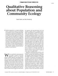
Geoinformation comprises spatial and thematic components. An effective system for qualitative reasoning about consistency in geoinformation, therefore, requires a representation that can encompass both spatial and thematic information. A series of publications by Randell, Cui, and Cohn has developed the well-known region connection calculus (RCC) and explored its application to spatial regions (e.g., [19,20]). While RCC is commonly used in the context of qualitative spatial reasoning, RCC is not explicitly spatial and may equally be applied to many non-spatial problem domains. For example, G¨ardenfors [21,22] has explored the application of RCC to reasoning about categorization in conceptual spaces. This paper takes these approaches a step further, integrating qualitative reasoning about both spatial and conceptual regions. The region connection calculus is based on work by Clarke [23] and assumes, as primitives, regions and a dyadic connection relation defined over those regions. The statement C(x, y) asserts that x is connected to y, and is axiomatically reflexive and symmetric. Intuitively, the statement ¬C(France, England) asserts that the spatial region France is not connected to the spatial region England (the two spatial regions are separated by the English channel). Similarly, the statement C(woodland, forest) asserts that the thematic region woodland is connected to the thematic region forest (i.e. the category or theme woodland has some overlap with the category or theme forest). 4
¬ Cs(x,y)
Cs(x,y)
Thematic
x y
y
x
Ct(x,y)
x
x
¬ Ct(x,y)
y
y Spatial
Fig. 1. Spatio-thematic connection in geographic regions
A geographic region can be represented as the combination of its spatial extent (the physical space that the region occupies) and its thematic extent (the conceptual space that the region occupies). Representing a geographic region’s temporal extent may also be important, but is not directly considered in this paper (but see §7). For a pair of geographic regions, we might ask whether 1) the spatial extents and 2) the thematic extents of the regions are connected. Ideally, spatially connected regions from related geographic data sets will also be thematically connected. Because of the inherent uncertainties in geoinformation, often this ideal relationship does not hold (and hence, inconsistencies arise). Using the notion of connection provides a convenient, unified representation that can support qualitative reasoning about both the spatial and thematic aspects of geoinformation. From this point onward we use the subscripts s and t to distinguish between spatial and thematic relations: Cs (x, y) asserts that two geographic regions x and y have a connected spatial extent, while Ct (x, y) asserts that they have a connected thematic extent. Whilst we will return to the RCC later on in this paper, the following sections are concerned solely with Clarke’s original calculus of regions and their connections. Figure 1 summarizes the four possible combinations of spatial and thematic connection between two geographic regions. Each box in figure 1 contains two geographic regions. Each region is shown in two-dimensions, with one spatial dimension (the x-direction) and one thematic dimension (the y-direction). For example, the two regions in the top right hand corner are not spatially connected (they do no overlap in the x-direction), but are thematically connected (they overlap in the y-direction). This situation is akin to the relationship between a French woodland and an English forest: they overlap thematically, but are spatially disjoint. 5
3.1 Simple spatio-thematic knowledge base Armed with a representation of spatio-thematic connection between geographic regions, it is possible to begin to write down a very simple knowledge base aimed at reasoning about consistency in geographic regions. For example, the three rules below provide definitions for consistent, possibly consistent, and inconsistent geographic regions. All three rules concern the spatial and thematic connection, Cs and Ct , between pairs of geographic regions, x and y, drawn from two different (data) sets X and Y . It is important to note at the outset that these rules are intended to provide a plausible example of how consistency can be represented, but not a universal definition of consistency. In later sections we develop more sophisticated models of consistency.
3.1.1 Consistent The first rule in equation 1 states that a geographic region x ∈ X is defined as consistent with respect to the set Y of geographic regions, written ConY (x), if it is spatially connected to at least one geographic region y ∈ Y , and is thematically connected to all regions to which it is spatially connected. In essence, consistent regions always agree spatially and thematically.
∀x ∈ X.ConY (x) ↔ ∃y ∈ Y.Cs (x, y) ∧ ∀y ∈ Y.Cs (x, y) → Ct (x, y)
(1)
3.1.2 Possibly consistent The second rule in equation 2 states that a geographic region x ∈ X is possibly consistent with respect to Y , written PosY (x), when it is thematically connected to some geographic region to which it is spatially connected. In essence, possibly consistent regions agree spatially and thematically at least some of the time.
∀x ∈ X.PosY (x) ↔ ∃y ∈ Y.Cs (x, y) ∧ Ct (x, y)
(2)
3.1.3 Inconsistent The third and final rule in this simple knowledge base describes when a geographic region x ∈ X is inconsistent with respect to Y , written IncY (x). The rule might simply be the converse of Equation 1, i.e., ∀x ∈ X.IncY (x) ↔ ∃y ∈ Y.Cs (x, y) ∧ ∀y ∈ Y.Cs (x, y) → ¬Ct (x, y), where an inconsistent region is thematically connected to none of the geographic regions to which it is spatially 6
connected. However, a simpler equivalent rule, in equation 3 below, can be achieved using the negation of the possibly consistent rule above.
∀x ∈ X.IncY (x) ↔ ¬PosY (x) ∧ ∃y ∈ Y.Cs (x, y)
4
(3)
Reasoning system
The discussion in §3.1 introduced some plausible first-order logical rules that might be used to describe consistency for two geographic data sets, as a first step toward integrating these data sets. While the rules above are plausible, they are not unique and might not be appropriate for some data sets or applications. It is to be expected that the semantics of particular applications may demand different knowledge bases. Further, many applications will require more sophisticated representations of connection, more complex rules, and a more sophisticated representation of consistency. Some such examples are discussed in later sections. Consequently, the aim in this paper is to be able to encode plausible rules within a reasoning system in such a way that the knowledge base can be independently extracted, examined, and updated. There exists a wide variety of knowledge-based reasoning systems that might be used for this purpose. Automated reasoning systems can be classified into four categories: logic programming languages, production systems, frame systems, and semantic networks; and description logics ([24] p297). All of these types of reasoning system have at some point been used in the context of geoinformation. Egenhofer and Frank [25], for example, address the integration of logic programming and spatial databases. To date, relatively few studies have applied description logic to reasoning about geographic information (e.g., [26] on reasoning about spatialtemporal regions and [27] on intensional definitions of geographic ontologies using description logics). A feature of any reasoning system is that it must strike a compromise between expressiveness and inferential power. While unrestricted first order predicate logic is highly expressive, it is not useful for efficient inference as it is generally not decidable and often not tractable. The reasoning system described in this section is based on description logics, which lie toward the opposite extreme. While offering rather limited expressiveness, description logics provide powerful yet decidable and tractable inference. 7
Expression
Syntax
Top
⊤
Bottom
⊥
Concept name
A,B
Concept conjunction
A⊓B
Concept disjunction
A⊔B
Concept negation
¬A
Role name
P ,Q
Role conjunction
P ⊓Q
Role negation
¬P
Universal quantification
∀P.A
Existential quantification
∃P.A
Table 1 A description logic expression syntax
4.1 Description logic
A formal introduction to description logics can be found in a wealth of literature on the subject. Brachman and Schmolze [28] describe the KL-ONE language, from which contemporary description logics are descended. More recent overviews of reasoning with description logics can be found in Donini et al. [29] and Calvanese et al. [30]. Rather than attempt a lengthy formal introduction here, only the key features of description logics are informally outlined in this section. Description logics are decidable, tractable fragments of first order predicate calculus. As suggested above, description logics achieve decidability and tractability at the expense of expressiveness. Expressions in description logic concern monadic predicates (called concepts), dyadic predicates (called roles) and some associated operations and quantifications over these concepts and roles. Description logics differ in exactly which operations and quantifications they support. Table 4.1 gives the syntax for a description logic expressive enough to be used to implement the simple knowledge base in §3.1. This syntax is in fact a subset of the syntax for the so-called ALB description logic described in [31]. It is now possible to begin to rewrite the simple knowledge base constructed in §3.1 using description logic syntax. The possibly consistent rule, PosY in equation 2, can be rewritten using the ALB description logic syntax as the set of individuals (geographic regions) for which the intersection of the roles 8
Cs and Ct is not empty, as in equation 4 below. In other words, a region is possibly consistent with respect to a set of geographic regions Y if there exists a region y ∈ Y to which it is both spatially and thematically connected. The roles Cs and Ct are primitive, in the sense that they are not defined in terms of any other concepts or roles in the logic. In many description logic systems it is possible to define the properties of roles, for example to define Cs and Ct as reflexive and symmetric, but for now we ignore such features. . PosY = ∃(Cs ⊓ Ct ).Y
(4)
The description logic expression for inconsistency, IncY , follows directly from the original first order predicate logic expression in equation 3 and the discussion above, as in equation 5 below. . IncY = ¬PosY ⊓ ∃Cs .Y
(5)
The definition of consistency ConY can be represented in description logic syntax by rewriting equation 1 using the conjunction of Cs and ¬Ct as in equation 6 (i.e. equation 1 is logically equivalent to ∀x ∈ X.ConY (x) ↔ ∃y ∈ Y.Cs (x, y) ∧ ¬∃y ∈ Y.Cs (x, y) ∧ ¬Ct (x, y)). . ConY = ∃Cs .⊤ ⊓ ¬∃(Cs ⊓ ¬Ct ).Y
(6)
4.2 Reasoning services
The benefit of expressing the simple knowledge base introduced in §3.1 within a description logic syntax is the ability to use four powerful reasoning services, provided by every description logic. Again, for a formal discussion of these reasoning services the reader is directed to [29], but an informal description follows. First, concept satisfiability is a reasoning service that can be used to determine whether a particular concept can be satisfied within the knowledge base. The concept IncY ⊓ PosY , for example, is not satisfiable (cf. equation 5). Second, description logic systems can check for coherence, and determine whether the expressions in the knowledge base lead to any contradictions. Third, subsumption solves the problem of checking whether one concept is necessarily more specific than another. Subsumption enables a description logic system to automatically classify the concepts defined in a knowledge base. For example, in the knowledge base above, PosY subsumes ConY , since every object that is ConY is also PosY . Further, ¬PosY subsumes IncY : everything that is inconsistent with respect to Y is not possibly consistent with respect 9
I
II
III
aI
Thematic extents
a A
bII b
A4
A1
g III
B
g B3 4
B2 3
2
1
Spatial extents Fig. 2. Consistency in abstract data sets
to Y . Fourth, description logic provides instance checking, described in more detail below.
4.2.1 Abstract data set The three reasoning services, satisfiability, coherence, and subsumption, concern qualitative reasoning about the general properties of the terms used in the system. The final reasoning service, instance checking, concerns reasoning about whether a particular object is an instance of a concept. An illustrative abstract data set is shown in figure 2. The data set consists of geographic regions with one-dimensional spatial extents and one-dimensional thematic extents for simplicity. As for figure 1, spatial extents are shown in the x direction, with thematic extents shown in the y direction. Geographic regions in the first data set, labeled using the bottom and right hand axes, have spatial extents 1, 2, 3 and 4 and thematic extents A and B. Geographic regions in the second data set, labeled using the top and left hand axes, have spatial extents I, II, III and thematic extents α, β and γ. The first data set X contains four geographic regions, shown using a dashed line and filled gray and labeled using a combination of their thematic and spatial extent labels, X = {A4, B3, B2, A1}. The second data set Y contains three geographic regions, shown using an unfilled strong unbroken line and similarly labeled, Y = {αI, βII, γIII}. The reasoning system can now be supplied with information about the connection between individual geographic regions in X and Y . For example, from figure 2 statements Cs (A4, αI), Ct (A4, αI), ¬Cs (A1, βII) and ¬Ct (A1, γIII) 10
all evaluate to true. Using instance checking, the description logic system can now derive those geographic regions in Y that are consistent with respect to X (βII), possibly consistent with respect to X (αI, βII, γIII) and inconsistent with respect to X (no regions); and those geographic regions in X that are are consistent with respect to Y (A4, B2), possibly consistent with respect to Y (A4, B2, B3), and inconsistent with respect to Y (A1). By omitting the formal details, the discussion in this section can only hope to provide a relatively superficial account of description logics and their reasoning services. Nevertheless, the discussion above does illustrate the key features of using a description logic reasoning system for determining consistency in geographic data set. Despite its restricted expressiveness, the description logic ensures the consistency of the knowledge base itself can be safeguarded (consistency and concept satisfiability); enables queries concerning individual geographic concepts or regions to be efficiently answered (instance checking); and provides an automated classification system for the concepts used in the knowledge base (subsumption).
5
Extending the reasoning system
Having explored a simple abstract example of reasoning about consistency in geoinformation using description logic, it is possible to move toward a more sophisticated example. The example considered in this section extends the simple example above in two ways. First, the effects of granularity upon consistency in geographic data sets are considered. Second, the RCC is used to differentiate between different types of connection in geographic regions.
5.1 Granularity and consistency
Imprecision concerns a lack of detail or specificity in a representation, and is an inherent feature of geoinformation. Imprecision leads to granularity: the existence of “clumps” or “grains” in information, where individual elements within a given grain cannot be discerned apart. The introduction of imprecision (often termed granulation) can lead to inconsistency between different information sources. Data sets may exhibit discrepancies as a result of imprecision, even if they are wholly accurate observations of crisp (i.e. not vague) features. Figure 3 illustrates the effects of accurate but granular observations of crisp reality. The two different observations, A and B, give rise to results that exhibit significant inconsistency. The inconsistency 11
Granular observation A Inconsistency (indicated as hatched region)
Crisp reality
Granular observation B
Fig. 3. Granularity and inconsistency
Fine granularity
Coarse granularity
Fig. 4. Consistent changes in granularity
introduced by the two granulations is shown as the hatched region on the right hand side of figure 3. Qualitative knowledge concerning the relative granularities of different geographic data sets may have important implications for consistency in those data sets. For example, by definition we expect finer granularity representations to contain more detail than coarser granularity representations of the same geographic phenomenon. Conversely, if a coarser granularity representation contains some detail that is not contained within a finer granularity representation of the same phenomenon, then we might assume that the two representations are inconsistent. To illustrate, figure 4 shows two small portions from two Ordnance Survey maps of Whitehall in central London at different granularities. The maps are scaled so as to have matching extents, but the finer granularity map is derived from the 1:10,000 scale map series, while the coarser granularity map is from the 1:25,000 map series. As expected, the fine grain map contains some detail not present in the coarse grain map, such as shapes of buildings and additional 12
Fine granularity
Coarse granularity
Fig. 5. Inconsistent changes in granularity
streets. Despite these differences, the two maps would still usually be thought of as consistent with each other, since our qualitative knowledge about the relative granularities of the two maps provides an adequate explanation of the differences. Such contextual knowledge can have a profound effect upon our understanding of the information presented. In figure 5, the fine granularity map has been deliberately manipulated to remove detail on the two government buildings (the Treasury and the Foreign Office) in the center of the image. The existence of more detail in the coarse granularity map is not what would usually be expected, and as a result, the differences between the two maps begin to take on a new significance as an inconsistency between the maps. It should be emphasized that while the example above uses two related cartographic map products (both maps are in fact derived from the same underlying survey data), this is just one illustration of the more general principle that qualitative information about relative granularity impacts our understanding of any geoinformation. Further, granularity is an inherent feature of all geoinformation, both as the unintentional consequence of the limitations of our measurement systems and as the intentional consequence of our desire for more effective representations of space (for example when geoinformation is simplified) [32]. Thus, granularity in geoinformation is unavoidable, and not simply an issue of the choice of data capture method (e.g., remote sensing versus ground survey) or representation (e.g., vector versus raster data structures).
5.2 Using RCC5
In the discussion above, qualitative knowledge about relative granularity is important for understanding the consistency of two data sets. Discrepancies between two data sets can be interpreted as inconsistencies or not, depending on the relative granularities. Qualitative knowledge of relative granularities is common in practical situations. Some authors have proposed detailed descrip13
EQs(x,y)
PPIs(x,y)
PPs(x,y)
POs(x,y)
DRs(x,y)
EQt(x,y) PPt(x,y)
Thematic
PPIt(x,y) POt(x,y) DRt(x,y)
Spatial Fig. 6. Spatio-thematic RCC5 connection in geographic regions
tions of how qualitative knowledge about granularity might be formalized (for example, [33,34]). However, here we assume only that the relative granularity of two regions is known. In order to take advantage of qualitative knowledge about granularity, it is necessary to adopt a more sophisticated representation of connection between two geographic regions. Based on connection, the RCC5 is able to distinguish five different types of connection relations between regions: distinct region (DR), partial overlap (PO), proper part (PP), proper part inverse (PPI) and equals (EQ). It follows that there exists twenty-five possible RCC5 relations between two geographic regions with spatial and thematic extents. Figure 6 extends the simpler diagram in figure 1 and enumerates the twenty-five possible relations that can be distinguished using RCC5. Qualitative knowledge about granularity can be used to decide whether one geographic region is of a spatially finer or coarser granularity than another. For simplicity, we assume here that only two granularities are possible. Correspondingly, we define new primitive concepts: Coarse, for regions at relatively coarse granularities; and Fine for regions at relatively fine granularities, where Coarse ↔ ¬Fine. It is now possible to write a revised rule for possibly consistent Pos′Y as in equation 7. The concept Pos′Y extends PosY (i.e. Pos′Y subsumes PosY ) by including any relatively fine spatial granularity regions that are proper part of a coarse grained region from which they are thematically disjoint. Previously, in the knowledge base developed in §3.1, such regions would have been classified as inconsistent. The intuition behind such a rule 14
is we expect fine grain regions to contain some detail not present in a coarse grain regions. Where discrepancies between regions can be accounted for on the basis of relative granularities, the regions are then classified as possibly consistent rather than inconsistent.
. Pos′Y = ∃(P Ps ⊓ DRt ).(Coarse) ⊔ ∃(Cs ⊓ Ct ).Y
(7)
For completeness, equation 8 gives the amended rule for the concept inconsistency, Inc′Y .
. Inc′Y = ¬Pos′Y ⊓ ∃Cs .⊤
(8)
The extension of the knowledge base, to include RCC5 relations and information about relative spatial granularities, can allow a much wider range of consistency concepts to be expressed. At the same time, while such rules when expressed in a description logic are guaranteed to be decidable and tractable, most non-specialist users might not expect to be able to formulate such rules. Since the rules already introduced are only intended as example constituents of a plausible knowledge base, it is important that non-specialist users should be able to formulate such rules. Consequently, the next section looks at the development of a flexible user interface to the knowledge base and illustrates how such an interface might help in an example application.
6
Example implementation and application
The discussion above (§3–5) provides a framework for automated reasoning about the consistency of geographic data sets based on the connection between geographic regions. Consistency issues are particularly important when attempting to fuse, integrate, or conflate two or more heterogeneous data sets. Information integration and interoperability are especially important topics for geoinformatics, where economies of scale demand high levels of reuse of geoinformation [35,36]. Any attempt to integrate heterogeneous geographic data inevitably generates a great many inconsistencies. The software described below is able to assist users in identifying inconsistencies in both the syntax and the semantics of the application data, and as such represents an important component of an interoperable system. 15
6.1 Software architecture
There a several different knowledge representation systems based on description logics that are now available, such as CLASSIC [37], CICLOP [38], and RACER [39]. Unfortunately, none of the implementations currently available are able to offer enough expressiveness for the example knowledge base discussed in §4 and 5 (the description logic ALB discussed in §4.1 has no corresponding implementation). Specifically, role conjunction is not yet supported by any of the implementations investigated. It is reasonable to regard this as a temporary situation. Description logic implementations inevitably lag a little behind theoretical work and there is a strong trend to incorporate more and more expressive reasoning into software implementations. Further, role conjunction syntax and semantics are included in the Knowledge Representation System Specification (KRSS, [40]), from which most implementations are derived. Given that role conjunction is not currently a feature of description logic implementations, RACER was chosen as the most suitable knowledge representation system for the application described below. RACER uses a distributed architecture, enabling clients to access remote reasoning services via a Java API. The user interface for a Java client developed for this purpose is described in §6.2. To combat the lack of role conjunction services in RACER, any role conjunction had to be performed outside RACER by the Java client. Based on 5 spatial and 5 thematic RCC relations, 25 new primitive roles were defined which described the conjunction of each spatial and each thematic RCC5 role (e.g., P Os DJt would be the role for geographic regions that partially overlap spatially and thematically disjoint). This rather inelegant solution would be unnecessary in future description logic engines that implement the full ALB logic.
6.2 User interface
In §3.1 and §4 it was noted that a consistency knowledge base was likely to be somewhat application-dependent. Description logic was adopted as a basis for reasoning about consistency, because it can help ensure that applicationspecific knowledge bases are coherent and it provides known decidability and tractability properties. As a result, the user interface developed to allow access to the reasoning system has two key goals: simplicity and interactivity. The user interface must help simplify the task of building and using an applicationspecific consistency knowledge base; offer the ability to dynamically refine the knowledge base; and enable users to observe the effects of changes in the knowledge base upon the ultimate consistency of the integrated data. 16
Fig. 7. Visual expression builder
With these goals in mind, the user interface for the reasoning system was based on a visual expression builder shown in figure 7. The main component of the visual expression builder is the area in the center of the user interface which is reserved for the manipulation of two regions. Users can move, resize, and reshape the regions using a combination of mouse clicks and drags. The connection relation (spatial, thematic or spatio-thematic) between these two regions can be included in the definition of a concept (using the “commit” button). Other expression elements, such as connectives and quantifiers, can be accessed from simple pull-down menus. The interface is flexible enough to allow all the rules in §5 to be built without using the keyboard. Figure 7 shows the interface being used to define the Pos′Y concept from equation 7. The user can load or save a knowledge base using the “File” menu, enabling different users to share or adapt knowledge bases for use with different applications. The “Write” button opens a connection to the RACER automated reasoning server, and writes the current knowledge base to the server. Users can access the visual expression builder at any time, make changes to the knowledge base, and propagate those changes through to their integrated geoinformation.
6.3 Application background
The example application chosen to test the prototype software was the integration of two land cover data sets for a small region of the UK. The two data sets are related in that they provide two independently derived representations 17
of the same geographical area (Great Britain) and similar thematic information (the land cover at different locations across Great Britain). However, the data sets are starkly different in their intended uses and (consequently) their granularity characteristics.
6.3.1 CORINE land cover map of Great Britain The Land Cover Map of Great Britain 1990 (LCMGB) was produced by the United Kingdom Institute of Terrestrial Ecology (ITE) in response to increasing demand for such information from land-use planners and environmental professionals. The LCMGB data is derived from Landsat 5 Thematic Mapper (TM) data using an automated classification process (described in [41]) that distinguished between 25 different cover types. However, in its original format LCMGB does not conform to the European Commission CORINE (“Coordination of Information on the Environment”) project to map the land cover of every member state [42]. As a result, a second product has been developed, the CORINE Land Cover Map of Great Britain 1990, which does conform to CORINE specifications. The CORINE land cover map has a minimum mappable unit of 25ha and a land cover classification of 44 possible cover groups, of which only 33 apply in Britain at 25ha resolution. The process of generalizing the CORINE land cover map is described in [43]. The result of this process is a land cover map with slightly finer thematic granularity (25 original LCMGB land cover categories to 44 CORINE land use categories) but coarser spatial granularity (minimum mapping unit increased from 0.125ha to 25ha).
6.3.2 Ordnance Survey MasterMap Ordnance Survey MasterMap has been developed through the OS Digital National Framework (DNF) project. An important part of the implementation of DNF has been a re-engineering of the National Topographic Database (NTD) from one that was designed primarily for cartographic purposes to one which is better suited to a much wider range of activities [44]. At the heart of this concept lies the notion that Ordnance Survey digital mapping should provide a consistent national framework for referencing geoinformation and should be capable of complete integration with other external data sets [45]. MasterMap comprises large-scale data incorporating detailed topographic information and a unique digital identifier or Topographic Object Identifier (TOID) on each feature. Individual features are classified using attribute set, feature description attributes and feature codes. However, because MasterMap is essentially a derived product (in the first instance from NTD but ultimately from paperbased “basic-scales” mapping) the classification of features owes much to the classifications employed in the original surveys. The land cover feature classi18
fications found in MasterMap are essentially unchanged from those described by Harley in 1975 [46]. The two data sets, CORINE and MasterMap, provide an interesting contrast. The former is a relatively specialized land cover map, whilst the latter is a general purpose mapping product specifically aimed at integration with other spatial data products. Further, the data sets exhibit what might be termed “contravariant” granularities: CORINE has higher thematic but lower spatial granularity, whereas MasterMap has lower thematic but higher spatial granularity. An integrated CORINE/MasterMap data set is desirable in order to provide detailed CORINE land cover information, suitable for environmental and cadastral applications, but directly related to MasterMap UK base mapping, via the TOID unique feature IDs. As suggested above, a first step in integrating these two data sets is to identify any inconsistencies that exist between them. Using the reasoning system allows inconsistencies to be explicitly identified and managed during the integration process. Equally important, by providing users with the flexibility to interact with the reasoning system, users have the opportunity to gain some insight into the nature of any inconsistencies between the two data sets.
6.4 Application
In addition to the visual expression builder described in §6.2, two more user interface components were needed to support the land cover application, all coded using Java. First, the main application user interface can be used to import and display multiple geographic data sets in standard geographic data formats (currently GML or Shapefile). The interface offers simple spatial query, display, and indexing functions rather like a conventional GIS. A screen shot of the interface is shown in figure 8, complete with some sample Ordnance Survey MasterMap data. The second application interface component enables users to build a “semantic map” for two (or more) geographic data sets. In many cases this semantic map may already exist. For example, the relationship between land cover classes in the CORINE data set and the earlier LCMGB data set is defined by Fuller and Brown [43]. In the case of CORINE and MasterMap data, however, there is no similar known mapping. An important task in integrating the CORINE and MasterMap data sets, then, is to build this semantic map. This task requires interaction with the human user. The user interface in figure 9 allows users to build a semantic map between geographic data sets by first placing thematic regions in the interface using the menus, and then manipulating those thematic regions using the mouse. 19
Fig. 8. Spatial data interface showing sample MasterMap data
Figure 9 shows a partially completed semantic map, with two classes from the MasterMap data set (larger squares with darker boundaries) and one class from the CORINE (smaller square with paler boundary). From this semantic map, the system can deduce that the CORINE “Water body” class is a proper part of the MasterMap “Surface water” class, and is a distinct region from the MasterMap “Defined natural land cover” class. Individual classes within a data set (e.g., “Surface water” and “Defined natural land cover” in MasterMap) are always assumed to be distinct regions, and the semantic map interface enforces this constraint by preventing overlapping semantic regions from the same classification. Based on the spatial data, the semantic map, the consistency knowledge base, and qualitative knowledge about the relative granularities of the two data sets, it is now possible to query the consistency of the data sets via the reasoning system. While the knowledge base can be stored to file, the results of consistency queries are not persistently stored in a database or a file. Instead, they are dynamically computed by the reasoning system when they are requested by the user. The reasoning system dynamically computes responses to queries, so users can make changes to any of the three linked interface components (the visual expression builder described in §6.2, the spatial data interface, and the semantic map interface described above) at any time. Changes to the consistency knowledge base, additions of new data, or alterations to the semantic map are automatically propagated through to any query results. By querying the reasoning system across the entire study area it is possible to derive a “consistency map” for the two data sets. Figure 10 shows a screen 20
Fig. 9. Semantic map interface
shot of a small example consistency map, resulting from the simple knowledge base described in §5, and from the partially completed semantic map in figure 9. Inconsistent regions are shown in dark gray, possibly consistent (but not consistent) regions in mid-gray and consistent regions with light gray (the actual interface uses different colors). The “uncolored” areas contain spatial regions with themes which are not yet included in the semantic map. In fact the consistency map in figure 10 is a composite of two consistency maps: the consistency of CORINE data with respect to DNF, and the consistency of DNF data with respect to CORINE. Usually, the two consistency maps will agree. However, the two consistency maps are not always symmetric, and it may be the case that for some x ∈ X, y ∈ Y such that PosY (x) either ConX (y) or IncX (y). It is never the case that for some x ∈ X, y ∈ Y such that C(x, y) then ConX (y) and IncY (x) (this can be checked using the description logic satisfiability reasoning service). In producing a composite of the two consistency maps, for ease of display we show only consistency or inconsistency (not possible consistency) on the consistency map where two overlapping regions have different consistency classifications. As users build up the semantic map, more regions move from uncolored to colored. As the semantic map becomes more consistent, more spatial regions move from darker colors to lighter colors. Figure 11 shows a more complete consistency map for the entire study area. In this way, users can build up an application-specific semantic map to drive the geoinformation integration process. This semantic map will be based on both the user’s domain expertise 21
Fig. 10. Example consistency map
Fig. 11. Example consistency map
as well as an explicit understanding of the consistency of the integrated data set, gained from the dynamic consistency maps. 22
7
Discussion
The system described above offers two important advantages over conventional GIS when integrating geoinformation. First, it enables users to initiate a dialog with the system about the inconsistencies between the data sets being integrated. Dialog and negotiation was cited in §2.1 as an important factor in communicating uncertainty to users. Second, the architecture ensures there is no information loss from the system during information integration by deferring any inconsistency resolution until the last moment. In this respect, the integration effectively produces a virtual data set [47], where the results of data integration are dynamically constructed on demand. The architecture uses description logic as the basis for its reasoning system. The description logic ensures any rules in the knowledge base are decidable and tractable. Decidability and tractability are vital since both changes to the knowledge base and execution of the reasoning process take place at run time, and so cannot be assured by many common reasoning systems. Inevitably, there are some drawbacks. Using a description logic places severe restrictions on expressiveness, although the constant drive toward more expressive description logics is continuing to extend the range of expressions that can be supported. Further, even though the description logic ensures responses to queries are tractable, there is an inevitable computational cost to dynamically computing responses to queries. For large numbers of queries ranging over the entire data set, recomputing query responses can cause slight delays in the prototype that can lessen the interactive nature of the user interface. However, there are many optimizations that might be implemented to increase the response speed of the system. In addition to addressing these drawbacks, the research has suggested several avenues of further research, discussed below.
7.1 Region connection calculus
§5.2 indicated how using the RCC5 could help refine the simple connectionbased model used in §3. Further refinements to the approach outlined above could be achieved by adopting more sophisticated calculi. For example, the RCC8 is a boundary sensitive refinement of RCC5, and might be appropriate to use when it is necessary to distinguish between regions that are distinct but share (part of) a boundary (RCC5 relation DR, RCC8 relation EC—externally connected), and regions that are distinct and completely disconnected (RCC5 relation DR, RCC8 relation DC—disconnected). The RCC has also been extended to represent indeterminacy in regions, providing the so-called egg-yolk calculus [48]. Qualitative reasoning about indeterminacy in geographic regions is important in many applications, including land cover applications where 23
land cover classes are often vague (e.g., “Forest”). Indeed, the consistency definitions introduced in §3.1 have been constructed with semantics compatible with egg-yolk regions or three-valued logic, already commonly used to represent indeterminacy and uncertainty (e.g., Conss forms the “yolk” or “true,” P oss forms the “egg” or “indeterminate,” and Incs forms complement of the “egg” or “false”). The approach set out in this paper is not limited to using the RCC family of calculi. Within RCC, regions are not allowed to be empty [49]. This proved problematic in the land cover application when partially complete semantic maps contained many empty thematic regions, leading to the uncolored, unclassified areas in §6.4 and figures 10 and 11. To combat this problem, related calculi that do accommodate empty regions might be adopted, such as the 9intersection model of Egenhofer and Franzosa [50] or the CBM of Clementini and Di Felice [51].
7.2 Extensions to the reasoning system
The focus of this paper has been integrated qualitative reasoning about both the spatial and thematic dimensions of geoinformation. A natural extension of this approach is to look at qualitative reasoning with temporal information. Several authors have already addressed spatio-temporal phenomena using region connection calculus (e.g., [52,26]), so reasoning with spatial, temporal, and thematic regions together seems entirely feasible. The system described does not go as far as to actually integrate the two data sets. Based on the semantic map, it is not difficult to augment the reasoning system to actually perform the final data integration step (see [53]). The reasoning system is currently purely qualitative, but might further be extended by incorporating some quantitative elements. Many reasoning systems based on description logics do possess the ability to reason using concrete domains, such as integers and real numbers. This capability could be useful for further refining consistency rules, for example by setting a minimum area which must be spatially and thematically connected before a geographic region is consistent. Finally, in the specific land cover application developed in §6, the lack of any prior knowledge about the relationship between the CORINE and MasterMap data set means users were required to build their own semantic map. In general, the process of building a semantic map for two data sets can be complex and require human domain expertise. Related research has begun to successfully tackle problem of automating part or even all of the process of building the semantic map for geographic data sets [54]. 24
Acknowledgments This work was conducted with funding from the UK EPSRC, under grant number GR/M 56685, from the US National Science Foundation under grant number EPS-9984342, from the European Commission under the REVIGIS project, grant number IST-1999-14189, and from the University of Melbourne, under an Early Career Researcher Grant entitled “Fusion of uncertain geographic information using inductive inference.” The authors would also like to acknowledge helpful contributions of Nic Wilson and John Stell in developing the ideas set out in this paper as well as the contributions of three anonymous reviewers.
References [1] R. R. Yager, Modeling uncertainty using partial information, Information Sciences 121 (3–4) (1999) 271–294. [2] L. Cholvy, A. Hunter, Information fusion in logic: A brief overview, in: Qualitative and Quantitative Practical Reasoning (ECSQARU’97/FAPR’97), Vol. 1244 of Lecture Notes in Computer Science, Berlin, 1997, pp. 86–95, springer-Verlag. [3] D. Gabbay, A. Hunter, Making inconsistencies respectable: part 1 - a logical framework for inconsistency in reasoning, in: P. Jorrand, J. Keleman (Eds.), Foundations of Artificial Intelligence Research, Vol. 535, Springer-Verlag, Berlin, 1991, pp. 19–32. [4] D. Gabbay, A. Hunter, Making inconsistencies respectable: part 2 - meta-level handling of inconsistency, in: M. Clarke, R. Kruse, S. Moral (Eds.), Symbolic and qualitative approaches to reasoning and uncertainty (ECSQARU’93), Vol. 747 of Lecture Notes in Computer Science, Springer-Verlag, Berlin, 1993, pp. 137–144. [5] J. Jensen, A. Saalfield, F. Broome, D. Cowan, K. Price, D. Ramsey, L. Lapine, Spatial data acquisition and integration, UCGIS Research Agenda (1998). URL http://www.ucgis.org/priorities/research/research white/1998% 20Papers/data.html [6] C. Date, An introduction to database systems, 5th Edition, Vol. 1, Addison-Wesley, Massachusetts, 1990. [7] M. Egenhofer, A. Frank, Object-oriented modelling for GIS, URISA Journal 4 (2) (1992) 3–19. [8] P. Besnard, L. del Cerro, D. Gabbay, A. Hunter, Logical handling of inconsistent and default information, in: P. Smets, A. Motro (Eds.),
25
Uncertainty Management in Information Systems, Kluwer, Boston, 1997, Ch. 11, pp. 325–341. [9] M. Goodchild, A. Shortridge, P. Fohl, Encapsulating simulation models with geospatial data sets, in: K. Lowell, A. Jaton (Eds.), Spatial accuracy assessment: land information uncertainty in natural resources, Ann Arbor, Michigan, 1999, Ch. 14, pp. 123–130. [10] K. Reinke, G. Hunter, Communicating quality in spatial information: notification — the first step, in: W. Shi, M. Goodchild, P. Fisher (Eds.), Proceedings of the International Symposium on Spatial Data Quality, 1999, pp. 66–75. [11] M. Beard, B. Buttenfield, Detecting and evaluating errors by graphical means, in: P. Longley, M. Goodchild, D. Maguire, D. Rhind (Eds.), Geographical Information Systems, Vol. 1, Wiley, New York, 1999, Ch. 15, pp. 219–233. [12] W. Tobler, A graphical introduction to survey adjustment, Cartographica 16 (4) (1996) 33–42. [13] G. Heuvelink, Error propagation in environmental modelling with GIS, Research monographs in GIS, Taylor and Francis, London, 1998. [14] J. Newcomer, J. Szajgin, Accumulation of thematic map error in digital overlay analysis, American Cartographer 11 (1) (1984) 58–62. [15] S. Benferhat, S. Lagrue, O. Papini, Belief change: A brief overview, International Journal of Geographical Information Science 18 (4) (2004) 355–390. [16] Y. Saygin, O. Ulusoy, A. Yazici, Dealing with fuzziness in active mobile database systems, Information Sciences 120 (1–4) (1999) 23–44. [17] H. Guesgen, J. Albrecht, Imprecise reasoning in geographic information systems, Fuzzy Sets and Systems 113 (2000) 121–131. [18] O. Ahlqvist, J. Keukelaar, K. Oukbir, Rough classification and accuracy assessment, International Journal of Geographical Information Science 14 (5) (2000) 475–496. [19] A. Cohn, B. Bennett, J. Gooday, N. Gotts, Qualitative spatial representation and reasoning with the region connection calculus, GeoInformatica 1 (3) (1997) 275–316. [20] D. Randell, Z. Cui, A. Cohn, A spatial logic based on regions and connection, in: Proc. 3rd International Conference on Knowledge Representation and Reasoning, Morgan Kaufmann, San Mateo, 1992, pp. 165–176. [21] P. G¨ardenfors, Conceptual spaces: the geometry of thought, MIT Press, Cambridge, Massachusetts, 2000. [22] P. G¨ardenfors, M.-A. Williams, Reasoning about categories in conceptual spaces, in: Proc. International Joint Conferences on Artificial Intelligence (IJCAI), Morgan Kaufmann, Palo Alto, 2001, pp. 385–392.
26
[23] B. Clarke, A calculus of individuals based on connection, Notre Dame Journal of Formal Logic 23 (3) (1981) 204–218. [24] S. Russell, P. Norvig, Artificial Intelligence: a modern approach, Prentice Hall, New Jersey, 1995. [25] M. Egenhofer, A. Frank, LOBSTER: combining AI and database techniques for GIS, Photogrammetric Engineering and Remote Sensing 56 (6) (1990) 919–926. [26] V. Haarslev, C. Lutz, R. M¨oller, A description logic with concrete domains and a role-forming predicate operator, Journal of Logic and Computation 9 (3) (1999) 351–384. [27] F. Hakimpour, S. Timpf, Using ontologies for resolution of semantic heterogeneities in gis, in: 4th AGILE Conference on Geographic Information Science, Brno, Czech Republic, 2001. [28] R. Brachman, J. Schmolze, An overview of the KL-ONE knowledge representation system, Cognitive Science 9 (2) (1985) 171–216. [29] F. Dononi, M. Lenzerini, D. Nardi, A. Schaerf, Reasoning in description logics, in: G. Brewka (Ed.), Principles of Knowledge Representation and Reasoning, CSLI Publications, 1996, pp. 193–238. [30] D. Calvanese, G. De Giacomo, D. Nardi, M. Lenzerini, Reasoning in expressive description logics, in: A. Robinson, A. Voronkov (Eds.), Handbook of Automated Reasoning, Vol. 2, Elsevier Science, Amsterdam, 2001, Ch. 23, pp. 1581–1634. [31] U. Hustadt, R. Schmidt, Issues of decidability for description logics in the framework of resolution, in: R. Caferra, G. Salzer (Eds.), Automated deduction in classical and non-classical logic, Vol. 1761 of Lecture Notes in Artificial Intelligence, Springer-Verlag, Berlin, 2000, pp. 191–205. [32] H. Veregin, Data quality parameters, in: P. Longley, M. Goodchild, D. Maguire, D. Rhind (Eds.), Geographical information systems, 2nd Edition, Vol. 1, Longman: Essex, 1999, Ch. 12, pp. 177–189. [33] M. Worboys, Computation with imprecise geospatial data, Computers, Environment and Urban Systems 22 (2) (1998) 85–106. [34] M. Worboys, Imprecision in finite resolution spatial data, GeoInformatica 2 (3) (1998) 257–279. [35] A. Frank, W. Kuhn, Advances in spatial databases, in: M. Egenhofer, J. Herring (Eds.), Specifying open GIS with functional languages, no. 951 in Lecture notes in computer science, Springer-Verlag, New York, 1995, pp. 184–195. [36] M. Sondheim, K. Gardels, K. Buehler, GIS interoperability, in: P. Longley, M. Goodchild, D. Maguire, D. Rhind (Eds.), Geographical Information Systems, Vol. 1, Wiley, New York, 1999, Ch. 24, pp. 327–358.
27
[37] R. Brachman, D. McGuinness, P. Patel-Schneider, L. Resnick, A. Borgida, Living with CLASSIC: when and how to use a KL-ONE-like language, in: J. Sowa (Ed.), Principles of semantic networks: explorations in the representation of knowledge, Morgan Kaufmann, California, 1991, pp. 401–456. [38] F. de Bertrand de Beuvron, F. Rousselot, M. Grathwohl, D. Rudloff, M. Schlick, CICLOP, in: P. Lambrix, A. Borgida, M. Lenzerini, R. M¨oller, P. Patel-Schneider (Eds.), Proc. International Description Logics Workshop (DL-99), 1999, http://CEUR-WS.org/Vol-22. [39] V. Haarslev, R. M¨oller, Description of the RACER system and its applications, in: C. Goble, R. M¨oller, P. Patel-Schneider (Eds.), Proc. International Description Logics Workshop (DL-2001), 2001, http://CEUR-WS.org/Vol-49. [40] P. Patel-Schneider, B. Swartout, Description logic knowledge representation system specification from the KRSS group of the ARPA knowledge sharing effort, http://www.bell-labs.com/user/pfps/krss-spec.ps, accessed 28 December 2001 (1993). [41] R. Fuller, G. Groom, A. Jones, A land cover map of Great Britain: an automated classification of Landsat Thematic Mapper data, Photogrammetric Engineering and Remote Sensing 60 (5) (1994) 553–562. [42] M. Bossard, J. Feranec, J. Otahel, Corine land cover technical guide, Tech. rep., European Environment Agency, technical report No. 40 (2000). [43] R. Fuller, N. Brown, A CORINE map of Great Britain by automated means, techniques for automatic generalization of the Land Cover Map of Great Britain, International Journal of Geographical Information Science 10 (8) (1996) 937–953. [44] Ordnance Survey, Digital National Framework - an introduction, Tech. rep., Ordnance Survey, consultation paper 1/2000 (2000). [45] Ordnance Survey, Associating data with the Digital National Framework, Tech. rep., Ordnance Survey, consultation paper 5/2000 (2000). [46] J. Harley, Ordnance Survey Maps a descriptive manual, Ordnance Survey, Southampton, 1975. [47] A. Vckovski, Interoperable and distributed processing in GIS, Research monographs in GIS, Taylor and Francis, London, 1998. [48] A. Cohn, N. Gotts, The ’egg-yolk’ representation of regions with indeterminate boundaries, in: Burrough, P.A., Frank, A.U. (Eds.), Geographic objects with indeterminate boundaries, GIS Data 2, Taylor and Francis, London, 1996. [49] J. Stell, Part and complement: fundamental concepts in spatial relations, Annals of Artificial Intelligence and Mathematics 41 (1) (2002) 1–17.
28
[50] F. R. Egenhofer, M., Point-set topological spatial relations, International Journal of Geographic Information Systems 5 (2) (1991) 160–174. [51] E. Clementini, P. Di Felice, A model for representing topological relationships between complex geometric features in spatial databases, Information Sciences 90 (1–4) (1996) 121–136. [52] T. Bittner, Approximate qualitative temporal reasoning, Annals of Mathematics and Artificial Intelligence 35 (1–2) (2002) 39–80. [53] M. Worboys, M. Duckham, Integrating spatio-thematic information, in: M. Egenhofer, D. Mark (Eds.), Geographic Information Science, no. 2478 in Lecture notes in Computer Science, Springer, Berlin, 2002, pp. 346–361. [54] M. Duckham, M. F. Worboys, An algebraic approach to automated geospatial information fusion, International Journal of Geographic Information Science 19 (2005) in press.
29