Quantification of the severity and distribution of ... - Semantic Scholar

Tina Memo No. 2000-007 Short Version published in Proc. MIUA, p. 61-64, London, 10th-11th July 2000. Published in Radiology 224 p. 278-285, 2002.

Quantification of the severity and distribution of cerebral atrophy provides diagnostic information in dementing diseases. N.A. Thacker, A.R. Varma, D.Bathgate, J.S. Snowden, D.Neary and A.Jackson. Last updated 7 / 2 / 2002

Imaging Science and Biomedical Engineering Division, Medical School, University of Manchester, Stopford Building, Oxford Road, Manchester, M13 9PT.

Quantification of the severity and distribution of cerebral atrophy provides diagnostic information in dementing diseases. Neil A. Thacker1 (BSc,PhD), Anoop R. Varma2 (MD,MRCP), Deborah Bathgate2 (MBCMB,MRCP), Julie S. Snowden2 (BA, PhD), David Neary2 (MD,FRCP) and Alan Jackson1 (PhD,MRCP,FCRC) 1: Division of Imaging Science and Biomedical Engineering, Medical School, University of Manchester, Oxford Rd, Manchester, M13 9PT. 2: Cerebral Function Unit, Manchester Royal Infirmary, Oxford Rd, Manchester, M13 9WL, UK.

Abstract Purpose: The currently accepted view on the use of MRI in dementing disease is that it has little role to play in the diagnostic process. The hypothesis here is that this assertion is wrong. Materials and Methods: We show here how a reliable and fully automatic image analysis system is feasible which can provide a simple yet powerful analysis of the distribution of cerebrospinal fluid. The technique has been tested on a mixed group of 57 subjects. Analysis was performed using a combination of image processing segmentation and statistical classification techniques. All manual stages were performed by two independent operators in order to eliminate user error and to evaluate reproducibility. Results: The results indicate that this distribution, once corrected for normal ageing and head size, is highly characteristic of Fronto-temporal (FTD), Alzheimers (AD) and Vascular dementias (VD). The technique described here identified FTD patients from a population of AD and FTD with a sensitivity of 79 % and specificity of 72 % rising to 82 % and 92 % respectively after application of an 80 % probability threshold. These performance figures support the use of this approach as a diagnostic tool to help identify demented patients in whom a diagnosis of AD should be reviewed. Conclusions: Volumetric analysis of the distribution of cerebrospinal fluid provides a source of valuable information for diagnosis of dementing disease which is complementary to standard diagnostic practices. Key words: automated analysis, atrophy, dementia, Magnetic Resonance Imaging, cerebrospinal fluid,

2

Introduction Cerebral atrophy is a non-specific finding which can result from brain injury or degeneration and which occurs normally in ageing. Many disease processes result in a distinctive patterns of atrophy due to differential involvement of different areas of the brain [1, 2, 3, 4]. In some diseases (such as olivopontocerebellar degeneration) the pattern of atrophy demonstrated on neuroimaging can be so distinctive that it forms a major component of the diagnosis [5]. However, this is not invariably the case. In other disorders, such as Alzheimer’s disease (AD), the pattern of the atrophic process is close to that of normal ageing, albeit at an accelerated rate [1, 6]. In clinical practice cerebral atrophy is most commonly assessed subjectively by the radiologist, who attempts to identify any specific areas of focal atrophy which might be of diagnostic value and to gauge whether the overall degree of global atrophy is appropriate for the patients age. In fact it is clear that subjective assessments of this type are unreliable and poorly reproducible [4, 7, 8]. Many approaches have been taken to improve the assessment of cerebral atrophy, particularly in elderly subjects where normal age related atrophy makes the interpretation of imaging findings particularly difficult. Despite this, existing techniques tend to be overly simplistic, with poor reliability and reproducibility [9, 10] or computationally expensive and time consuming [11]. These latter, more complex methods can provide valuable information concerning the natural history of individual diseases but are too complex for diagnostic use in a clinical environment. We present here a new technique for the assessment of cerebral atrophy from magnetic resonance (MR) images. The technique was designed to be simple to implement, highly reproducible and to provide a generic approach for the assessment of both the pattern and severity of atrophy in any brain disorder. In order to meet these design objectives we have chosen to use measurements of cerebrospinal fluid (CSF) volume as an indicator of atrophy. The use of the CSF space as the primary indicator of brain loss allows the use of robust segmentation tools since the characteristics of CSF on MR images are highly distinct. In addition the CSF space reflects the pre-morbid head size and allows automatic correction of individual variability. In order to obtain information about the distribution of atrophic changes we use a stereotaxic co-ordinate system based on the dimensions of the CSF space, which is then divided into 12 equal- sized volumes. These volumes are defined by dividing the volume into anterior, middle and posterior thirds and subdividing these by placing horizontal and vertical sampling planes centrally from anterior to posterior. The proportion of CSF in each of these volumes is then normalised and corrected to remove variations due to head size and age-related effects due to normal atrophy and used to derive 5 independent variables (W1-W5). These variables represent the age corrected relative degree of atrophy between: middle and front of the CSF space (W1); middle and back of the CSF space (W2); left and right sides (W4) and top and bottom (W5). The remaining variable (W3) is a measure of the overall relative degree of atrophy. These variables represent a rotation in the original space chosen such that correlations between the variables are effectively eliminated in all but W3. This technique was designed with the intention of providing an automated analysis tool that could be used in a clinical environment to provide supportive information for diagnostic decisions. The work presented here is intended as a proof of concept study to establish the ability of this analytical approach to discriminate between normal subjects and patients with three different dementing disorders (AD, frontotemporal dementia (FTD) and vascular dementia ( VAD) on the basis of simple CSF volumetric measurements.

Methods Patient Selection and Clinical Diagnosis. The subjects comprised 19 patients with frontotemporal dementia, 18 with Alzheimer’s disease, 11 with vascular dementia and 9 normal controls. Their age distribution and duration of illness are shown in table 7. All patients were referrals to a specialist diagnostic dementia clinic, and had undergone comprehensive

1

neurological and neuropsychological assessments as part of their diagnostic evaluation. Patients with frontotemporal dementia and Alzheimer’s disease fulfilled currently accepted clinical diagnostic criteria for those conditions [12, 13, 14] and were free from significant risk factors for cerebrovascular disease (Hachinski scale < 4) [15]. Patients with vascular dementia all had high risk factors for vascular disease, with Hachinski scale scores > 7. Patients exhibited the characteristic pattern of dementia associated with their clinical diagnosis [16]. All patients had been followed up for 1 − 3.5 years. The clinical diagnosis was therefore confirmed by the evolution of the illness. Individuals were excluded if diagnosis of the form of dementia was equivocal or if the clinical pattern suggested mixed aetiology.

Imaging All subjects were scanned using a Phillips 1.5 Tesla ACS-NT scanner with a PowerTrack 6000 gradient subsystem. The patients were scanned using a birdcage headcoil receiver. CSF segmentation was performed on coronal fast spin echo inversion recovery images (TR 6850 ms, TE 18 ms, TI 300 ms, echo train length = 9 ). Contiguous 3mm slices were obtained throughout the brain with an in-plane resolution of 0.89 mm2 (matrix 256 x 204, field of view 230mm x 184mm ).

Image Processing Images were analysed a slice at a time using the TINA machine vision software [17, 18] in order to automatically identify the CSF spaces in the images. This was done using derivative based techniques (similar to the Canny edge detector) to extract the edges between the CSF and other tissues and setting a threshold at the mean grey level value of the corresponding edge pixels. The image data was then binarised, labelling CSF data with a one and non-CSF tissues with a zero. The binary data was then manually edited to delete the eyes and sinuses leaving only CSF volumes within the brain cavity. The original volume was manually rotated using sagittal, axial and coronal slices from within the MR volume. The axes of symmetry of the brain in the coronal and axial views were aligned to the vertical and horizontal planes. The mid-sagittal slice was then rotated to align the horizontal axis with the ventral surface of the genu of the corpus callosum and the junction of the of the corpus callosum with the body of the fornix. The limits of the CSF space were automatically identified as the extrema in all directions (Plef t , Pright , Pupper , Pf ront , Pback ) except for the lowest Plower . This was defined by drawing a line in the mid sagittal slice parallel to the horizontal axis passing through the junction of the calvarium and the tentorium cerebelli. Twelve CSF volumes were measured by dividing the brain in half top to bottom, left to right and in thirds front to back. We then normalised these measurements by dividing by the total rectangular volume (Plef t − Pright ).(Pupper − Plower ).(Pf ront − Pback ) in order to arrive at estimates which were independent of head size. All manual stages of processing were duplicated by two researchers in order to investigate the effects of inter-observer variability and to eliminate gross errors in data management. We believe that the manual stages in this process could be automated by co-registration to a standard brain at the required orientation. The method thus forms the basis for a fully automated system. Although correlations could be sought between individual parameters and diagnostic factors, a set of twelve measurements would require a considerable quantity of data in order to investigate all possible correlations fully. We therefore selected the following set of seven derived variables: • F The normalised sum of the four front volumes. • M The normalised sum of the four middle volumes. 2

• B The normalised sum of the four back volumes. • P The normalised sum of the six volumes on the left side. • S The normalised sum of the six volumes on the right side. • U The normalised sum of the six upper volumes. • L The normalised sum of the six lower volumes.

Correction for Age Related Atrophy The data from normal subjects was used to derive a correction for the process of atrophy due to normal ageing. It was assumed that the normal development of atrophy in any of our pooled variables V would be of the form V = (age − C)/K Thus we can construct a new variable representing the proportion of atrophy relative to that expected at a particular age. V ′ = V K/(age − C) By taking the value of K to be (65 − C) we can centre this correction process around the age of 65 (approximately the mean of our data set) while at the same time leaving us with a single free parameter with which to model the process. Values of C were taken which minimised the variance in the corrected variable V ′ for the normal group. Typical age related corrections to the original measured variables were of the order of 10 %. The calibration factors and minimum deviations estimated for the age correction process in the normal group of subjects are shown in Table 1. These results indicate that normal age related atrophy has slightly greater effects in the dorsal regions of the CSF space than elsewhere. It is also seen that the age related correction in the upper region of the CSF space is less efficient than in other regions though this is not statistically significant with this sample size. From repeatability studies the age corrected variables were found to have the approximate characteristics of Poisson random variables ie: the data had increasing variance for larger measurements. This is consistent with a stochastic volume measurement process. These measures can thus be converted into measures which have uniform variance by taking the square root [19]. The set of seven square root variables should thus define a seven dimensional space with homogenous errors. However, residual intra-subject age differences, developmental effects and systematic measurement errors leave some residual correlations between these absolute factors. From these a reduced set of relative variables were constructed as described in the next section.

Effects of Variable Normalisation The variables selected were as follows; • The age corrected relative degree of atrophy between the middle and front of the CSF space. √ √ √ W1 = ( M ′ − F ′ )/ 2 • The age corrected relative degree of atrophy between the middle back of the CSF space. √ √ √ W2 = ( M ′ − B ′ )/ 2 3

• The age corrected relative degree of total atrophy √ √ √ √ W3 = ( F ′ + M ′ + B ′ )/ 3 • The age corrected relative degree of atrophy between the left and right sides of the CSF space.

√ √ √ W4 = ( P ′ − S ′ )/ 2 • The age corrected relative degree of atrophy between the top and bottom of the CSF space.

√ √ √ W5 = ( U ′ − L′ )/ 2 Table 2 shows the standard deviations of the rotated variables for the 18 (two observations per subject) normal subjects and an estimate of the reproducibility of the manual stages of the technique using the two sets of measurements for the entire group of 57 subjects. These results indicate that derivation of normalised variables has successfully eliminated the effects of subject related correlated errors in W1 , W2 and W4 . The remaining two variables, W3 and W5 , are significantly less reproducible. This is related to the absolute nature of the measure, which includes error terms arising from the manual specification of the lower limit of the CSF space. These errors represent upper limits on actual measurement performance. The reproducibility estimate is the accuracy for repeating the same set of measurements in the same subject. It therefore gives an indication of the ability to monitor the progression of atrophy. However, it is a best case estimate of measurement accuracy as it excludes any systematic variations in CSF segmentation. Subjects who differ by more than these quantities can be said to be measurably different even if the diagnosis is the same. The similarity between the scales of repeatability and standard deviations of the normal group is quite striking. The normal group has inter-group variations for which approximately half can be accounted for by measurement error. This factor could possibly be reduced by full automation of all stages of data processing Visualisation of multi-dimensional data is problematic. Before attempting a quantitative analysis of the data we used the package XGOBI to examine the data for strong correlations or diagnostic patterns. These variables were then used to construct a Parzen window classifier using the repeatability estimates to scale the probability kernel. The performance of this classifier was evaluated using a leave-one out cross-validation technique.

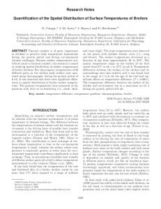
Results Comparison of Normalised Variables (W ) in Normal Elderly and Dementing Disorders. We will describe first the behaviour of the diagnostic variables (development of these variables is described in the Methods section). Comparison between normal elderly individuals and patients with AD, FTD and VAD shows clear evidence of disease related patterns of atrophy. A plot of W2 vs W3 (Figure 1 (a))(middle to back trend versus overall level of atrophy) shows very good separation for all four groups. The normal and vascular dementia groups form separated clusters of a size similar to the expected measurement accuracy. AD and FTD patients form more diffuse but quite cleanly separated groups which overlap only marginally outside of the normal brain distribution, indicating that the progression of atrophy follows different patterns in the two diseases. Normal elderly and VAD patients have a very similar (overall low) level of atrophy whilst AD and FTD systematically demonstrate greater degrees of 4

atrophy. FTD and VAD groups have proportionately greater degrees of atrophy in the middle of the CSF space compared to the back than is seen in AD and normal elderly subjects. A plot of W1 vs W4 (Figure 1(b) )(front to middle trend versus left right asymmetry) shows that normal elderly and VAD patients have similar levels of asymmetry which are individually consistent (within measured errors) with zero. Patients with AD have greater asymmetry than normal elderly and VAD patients. This may increase as overall atrophy progresses but show no obvious bias. The FTD group has the greatest levels of asymmetry with a definite bias to the left-hand side. AD patients show a stronger front to middle trend than the others, which are otherwise broadly similar. The last variable, W5 , shows no obvious discrimination capabilities when used in conjunction with other parameters though the distribution of this parameter between groups still does hold some residual information, with AD showing more specific atrophy at the top of the brain than the other groups and VAD showing relatively more atrophy at the bottom (Figure 1 (c)).

Diagnostic Performance of the Normalised Variables. The simple approach to the analysis of multi-dimensional data would be to compute mean and deviations for each group on the basis of an assumption that each set is drawn from a Normal distribution. This approach is not adequate here as visualisation of the parameter space demonstrates quite clearly that the group clusters are not Normally distributed. Therefore, in order to obtain a quantitative measure of separability of the data the repeatability measures from Table 2 were used to define the kernel for a Parzen classifier. Defined this way the classifier is computing the relative likelihood that each pattern can be considered to be consistent with each data class on the basis of measurement accuracy. The technique makes no assumptions regarding the underlying distributions except that the available data was representative and that measurement errors are Normal. In this analysis each subject is entered twice due to pooling of the data from the repeatability study. The first set of diagnoses (Table 3, excluding both data points from each subject as it is classified) represents a lower limit on classification performance. The nature of cross-validation depletes the information available for the classifier as each data point is classified in exactly the region where the data is needed. As a consequence, such measures of classifier performance, while giving a good indication of the spatial distribution of classes, often improve significantly with additional training data and represents a ”worst possible” outcome for automated classification. We have therefore followed the suggestion of other authors [20] and taken the average of the leave-one-out and leave-all-in classifcation results (Table 4) in an attempt to predict what may be possible with unlimited statistics. Tables 3 and 4 are useful for assessing the distribution and separability of our patient groups in the five dimensional classification space, but in clinical practice the most relevant issues are separation of AD and FTD and the diagnosis of early AD from normal elderly. The cross validated diagnosis from FTD and AD, calculated using a Parzen classifier with the same parameters as previously (but excluding variable W5 due to poor information content), is shown in Table 5. The overall classification rate for these groups is 76 %. We estimate that approximately half of the mis-classified cases are in the region close to the normal group and the other half are distributed close to the interface between the two groups at large overall atrophy levels. This is demonstrated by the reduction in misclassification obtained when a Bayes probability above 0.8 is demanded. For this 73 % of the data the classification rate rises to 87 %. The cross-validated diagnosis from normal elderly and AD, calculated using a Parzen classifier is shown in Table 6. Although the AD patients represent a young cohort (median age with relatively early disease the classification rate is 92 % rising to 95 % when a Bayes probability threshold of 0.8 is applied. These numbers have been obtained on the basis of the data sample available for this study. Adjustments would need to be made to the Bayes prior factors to allow for regional cohort differences before such classifications could be used in any specific clinical environment.

5

Discussion The commonest cause of abnormal atrophy due to dementia is Alzheimer’s disease (AD) [21, 22] which has been reported to account for 50 to 75 % of all dementias. A large number of structural and volumetric MRI studies have noted anatomic and structural changes accompanying AD, including variable degrees of generalised cortical atrophy and specific atrophy of medial temporal lobe structures, particularly the hippocampus. Many studies have examined the feasibility of using atrophy as a diagnostic indicator in clinical practice and a variety of measurement based techniques have been described which discriminate between patients with AD and normal subjects. Unfortunately, many of these methods fail to separate patients with AD from those with other disorders, such as vascular (VD) and frontotemporal dementia (FTD). Studies to assess the validity of atrophy measurements in mixed populations of dementing disease are uncommon. However, some authors have reported results which suggest that the distribution of atrophic change can offer diagnostic specificity between the dementing diseases [23, 24, 25]. One major problem with the introduction of quantitative volumetric measurement techniques into clinical practice is their complexity and the time required for image processing. Some groups have tackled this by attempting to define ”sentinel changes” which will allow the use of simple linear measurements to support diagnostic decisions [26, 27, 28]. One of the best documented of these is the interuncal distance, first described in 1986 by Le May et al [29]. Le May used the distance between the medial points of the curved uncus, as identified on trans-axial CT scans obtained at the level of the suprasellar cistern. When compared to a number of other potential indicators, the interuncal distance showed the greatest discriminatory power between normal subjects and AD patients. Despite this, the measurement was not considered a useful clinical indicator because of large overlaps between the normal and abnormal ranges. In 1991, Dahlbeck et al [28] used the same measurement derived from axial MRI and showed excellent discrimination between AD (minimum interuncal distance 34.0mm) and normal elderly subjects (maximum interuncal distance 25.6mm). This study prompted further examination of the interuncal distance and in 1993 Doraiswamy et al [30] published a normative study of 75 subjects between 21 and 85 years of age. Although they demonstrated variation with both age and sex they did not observe any value greater than 30mm and supported the suggestion that the interuncal distance may be useful as a diagnostic indicator. However, in 1993 two other groups reported results, which cast significant doubt on the diagnostic value of the interuncal distance. Early et al [31] found no correlation between the interuncal distance and the volume of medial temporal lobe structures in normal subjects and no difference in the interuncal distance between normal and AD. Howeison et al [9] did identify a difference but with significant overlap between groups. Interestingly, these workers also described significant measurement errors in the estimation of interuncal distance, particularly from axial images. In 1994, de Leon et al [10] and Laasko et al [32] both re-examined the validity of the measurement and found no evidence to support the use of the interuncal distance as a diagnostic index. These extensive studies of the interuncal distance as a potential diagnostic indicator illustrate many of the problems associated with the use of linear sentinel measures of this type. Wherever linear measurements are produced from 2D images there are several unavoidable sources of error inherent in the placement of the measurement points. Although these errors may be small it is essential that they be documented and used to estimate confidence limits for individual diagnostic decisions. These estimates of error will vary according to scanning angle, slice thickness, in-plane resolution, operator experience and other factors, demanding strict standardisation of scanning technique. These problems affect all potential linear measurements and although other ”sentinel measurements” have been suggested [27], none has been subject to the level of validation undertaken for the interuncal distance and, consequently, no such measurement has been adopted in clinical use. A more logical approach to the quantification of atrophy is to measure the volumes of cerebral structures from 3D image data however this requires accurate delineation of structure margins. This is commonly accomplished by manual tracing techniques (the medieval scribe approach), which is extremely time consuming. The accuracy of volume estimations using this type of technique is limited by the relationship between the size of the structure and the spatial resolution of the images from which the measurements are taken. Studies using measurements of small structures, such as the hippocampus, typically employ

6

voxel sizes less than 1mm x 1mm x 3mm and many use spatial resolutions greater than this. The acquisition of MR images with this level of spatial resolution will produce over 100 slices through the brain so that manual delineation of larger structures becomes impractical. One approach to this problem is to identify areas which are specifically involved in particular disease processes and which therefore provide strong discriminative ability. Measurement of these specific structures can then be used to give diagnostic guidance although data from other areas of the brain is ignored. In patients with AD there is a considerable body of evidence that atrophy of medial temporal lobe structures, particularly the hippocampus, entorhinal cortex and uncus occurs early in the disease and progresses up to 10 times faster than is seen in normal elderly subjects [6, 33]. Measurements of the hippocampal and entorhinal cortex volumes have been shown to distinguish patients with AD from normal individuals and from patients with depression and other neurodegenerative brain diseases with a specificity of over 95 % [23, 34, 35]. Unfortunately, medial temporal lobe atrophy is also a feature of other neurodegenerative diseases, particularly frontotemporal dementia [36, 24]. In this disorder, atrophy occurs in the medial and lateral temporal lobe structures and is accompanied by extensive volume loss in other areas, particularly the frontal lobes. Compared to patients with AD the brain in FTD tends to be more severely atrophic with atrophy affecting larger areas of the cortex [25, 37] and, although the loss of medial temporal lobe volume occurs it is proportionately less severe than is seen in AD [24]. In a recent study, Frisoni et al [24] compared the patterns of temporal lobe atrophy in AD and FTD. They found atrophy of the entorhinal cortex to be equally severe in both disorders but hippocampal atrophy to be more marked in AD. When compared to control subjects these measurements gave diagnostic sensitivities of less than 60 % for FTD and 80 % for AD, the ability to differentiate between the diseases was poor. These studies illustrate the problems associated with the use of marker sites such as the hippocampus to identify disease specific patterns of atrophy. Although one particular pattern of regional atrophy may have excellent discriminative capability between a specific disease state and normal subjects it may be mimicked by other disorders leading to poor specificity when attempts are made to apply it to mixed populations of patients in clinical situations. In order to avoid bias of this type it is desirable to develop a metric that reflects the overall pattern and severity of cerebral atrophy thus providing a generic indicator, which is applicable in any disease state. One approach to this is to develop techniques which automatically identify and measure a wide range of structures within the brain providing a spectrum of ”structure specific” volume measurements [11]. This approach is technically possible using the concepts of trained models to construct a probabilistic atlas of the relationships of certain key features within brain images. However, one weakness of trained models is their inability to cope with variation outside the initial training set of data. This means that the training set must include a sufficient range of variation to include all potential pathological sources of variation that would be observed within the population to which it would be applied. In practice this would mean the development of an extensive training set including examples of all atrophy patterns which might be identified in the patient population which is impractical. Another approach to providing a generic metric for the assessment of whole brain atrophy is to ignore the classical anatomical boundaries of specific structures and to examine changes occurring within an arbitary but reproducible data space. The simplest approach to this is the definition of ”standardised” planes based on anatomical markers within the brain. This approach is widely used for parcellation of the prosencephalon into approximate lobar samples for comparison studies [38]. This simple approach can be logically extended to allow the identification of any structural volume by transformation of the 3D image data into a standard sampling space where the spatial distribution of the structure within the space is known. This technique is widely used in functional imaging to allow pooling of imaging data from multiple individuals. The co-ordinate system most commonly used was described by Talairach and was designed for use in stereotaxic surgical procedures [39]. The co-ordinate system is defined by a midline sagittal plane passing through the brain’s axis of symmetry and an axial plane passing though the anterior (AC) and posterior (PC) commissures. The boundaries of the co-ordinate system are delineated by the extremes of the brain in each of the orthogonal directions allowing the application of simple linear re-scaling. Transformation of data from individual experimental subjects allows direct comparison of the

7

sites of activation. This same approach has been used by Andreasen et al [40] to automate the measurement of structural volumes in normal subjects and in patients with schizophrenia. The problem with these approaches is that they assume a fixed spatial relationship between the brain and the co-ordinate system and ignore any spatial distortion induced by the atrophic process. Whilst this approach may be acceptable in disorders, such as schizophrenia, where atrophic changes are relatively small and are not associated with any known spatial distortion it cannot be safely applied in other disease states. An alternative approach is to measure the degree and pattern of deformation which must be applied to the individual brain in order to force a match with a standardised or averaged brain which has itself been transformed into a standard data space [41]. This ”warping” process will define a complex transformation matrix containing a description of the severity and pattern of atrophy, which could be theoretically used for diagnostic purposes. In fact these warping techniques are complex and computationally expensive and have not as yet been applied to this type of classification task. The approach, which we have taken, is deliberately both simplistic and generic. We have identified a novel 3D co-ordinate space based on the size and shape of the cranial cavity identified by the segmentation of CSF from the data set. The use of this co-ordinate system to define sampling volumes removes any sampling bias and provides automatic normalisation for individual variations in head volume. The use of CSF as the marker tissue allows the use of simple and robust segmentation techniques, which will not be affected by disease related changes in grey and white matter properties. The use of the intracranial space as a basis for the co-ordinate system makes the technique highly generic and free from systematic errors that might result if spatial distortion of the brain were to result from specific disease processes. In this study the rotational co-ordinates of the data space were defined from structures identified within the brain. Implicit in this is the assumption that the brain’s axis of symmetry and the position of the horizontal baseline, which we have defined, do not suffer from spatial distortion within the co-ordinate space as a result of the disease process. In clinical practice we would aim to automate this transformation step by automated alignment of the intracranial cavity itself into the data space using surface matching or trained model based techniques. This approach would remove the requirement for manual editing of extra-cranial fluid structures such as the vitreous humour. We also anticipate that automation would also be likely to reduce measurement errors, which were expressed as inter-group variations in the current study (Table 2). The divisions of the data space used in the study were arbitrarily selected to provide approximately equal sampling volumes covering the entire prosencephalon. In practice the existence of different, disease specific, patterns of atrophy suggests that a more strategic distribution of sampling volumes may produce improvements in diagnostic specificity. The optimal sampling strategy is likely to be specific to the diagnostic classification being made although it seems likely that some modification of sample selection would improve results a wide range of atrophic patterns. One possible improvement would be the inclusion of a ”central” sample, which would specifically reflect ventricular involvement. The derivation of optimal sampling strategies would be best established by use of genetic algorithms, which require larger data sets than were available for the present study. Other potential improvements in discriminative performance include the segmentation of brain tissue to identify the relative severity and distribution of grey and white matter loss contributing to the overall atrophic pattern. Several workers have demonstrated that atrophy in AD results principally from loss of grey matter with sparing of white matter volumes [42, 43] whilst the pattern of atrophy in FTD appears to affect both grey and white matter to some extent [25, 44]. In clinical practice the diagnosis of the dementing disorders does not rely solely on imaging examination. In practice, diagnosis can be made with high confidence using a combination of clinical and neuropsychological assessment but only in centres with a high level of experience and expertise. When imaging is performed the most commonly utilised diagnostic technique is 99mTc HMPAO SPECT studies of cerebral blood flow which demonstrate different patterns of flow reduction in different dementing diseases. In 1997 George et al [22] published a commentary in the American Journal of Neuroradiology entitled

8

”Imaging the brain in dementia: expensive and futile?”. This was stimulated by the growing controversy regarding the low diagnostic yield of cross sectional imaging techniques in the dementing disorders and the potential cost implications of performing routine MR imaging in the growing population of dementia patients. After reviewing the evidence these authors concluded that the main benefits of cross sectional imaging at the present time were to rule out unsuspected disease and to continue to advance our understanding of the disease processes and their longitudinal development. They also identified the ability of medial temporal lobe measurements in AD to confidently identify normal (non atrophic) subjects, and to thus identify ”pseudodementia” due to depressive illness, as justification for the use of MR scanning in this patient group. These authors also point to the development of new therapeutic agents designed to halt the progression of AD as motivation for the development of new diagnostic indicators. It is of interest that they were unable to justify the use of MRI as a primary diagnostic tool. The methodology we have described has the potential to change this situation. The technique we describe here is capable of full automation and is sufficiently undemanding of computing resource to be routinely performed in all dementia investigation. The technique can automatically identify the most likely diagnosis and can assign a probability to it, which can be used to guide the clinician or researcher in the clinical diagnostic process. The technique showed good diagnostic performance in the patient groups which we studied, particularly when specific diagnostic questions were addressed. The technique identified AD patients from a mixed population of AD and normal age matched controls with a sensitivity of 95 % and specificity of 93 % which is equal or better to the best reported results using medial temporal lobe volume measurements from CT or MR [22, 24, 45, 46]. This performance was improved by applying a Bayesian probability threshold of 80 % to produce sensitivity and specificities of 97 %. When considering these diagnostic performances it is important to note that the AD patients in this study were young (age 49-73, median 61 years) and many had early disease (time from onset 2-8 years, median 3 years). This suggests that the technique that we describe could be of genuine use in clinical practice to confirm a suspected diagnosis of early AD. Similarly the use of probability thresholding will support the selection of appropriate patients for trials of new therapeutic agents. The ability of the technique to identify patients with FTD is also of clinical interest. The syndrome of FTD is less well recognised than AD and although the criteria for diagnosis have been well established [13, 12] they require additional specialist assessment which may be impractical in non-specialist centres. The technique described here identified FTD patients from a population of AD and FTD with a sensitivity of 79 % and specificity of 72 % rising to 82 % and 92 % respectively after application of an 80 % probability threshold. These performance figures support the use of this approach as a diagnostic tool to help identify demented patients in whom a diagnosis of AD should be reviewed. The standard method for probablistic data classification is based upon Bayes theory. This involves computation of conditional probabilities based upon a model assumption and then combination with prior terms. These prior terms establish the relative frequency of each model hypothesis and without them the classification result will be sub-optimal (in the Bayes sense), i.e. there will not be a minimum number of incorrect classifications across a sample group. In a clinical diagnostic task the prior probabilities are determined by the statistical make-up of the classified data sample. Use of prior probabilities therefore requires a solution to the additional problem of ensuring that over an extended period of time the prior probabilities reflect the true frequency of occurrence of cases. This process is often referred to as case adjustment. Beyond simple classification, any decisions based on these results should also be made on the basis of the Bayes risk, such that any treatment delivered is made in order to improve the prognosis of the patient, rather than just getting the diagnosis correct. For example, if the diagnosis is ambiguous between three possibilities but two can have the same treatment, then this should influence the patient management. Though ultimately we would like to hope that ambiguity would be rare in a useful system. We could build a system with fixed priors based on a national average. If one were intending to build an optimal fully automatic classification system we could envisage one which attempts to determine prior probabilities from the sample data as it arrives. However, if we accept that for moral reasons this data should be moderated by a medical expert, such a system might be considered inappropriate. It is 9

inevitable that the expert will be attempting to make sense of the delivered results in terms of his own experience, which will include his own (perhaps subjective) opinion regarding typical frequency (as it must, given the way that his experience is gained). Also, any system which will change its classification of the same data set over a period of time, due to the frequency of the other diseases, will complicate any experiential learning of the expert. These isssues both raise doubts as to the direct use of Bayes theory in clinical diagnosis. So the question arises: if we cannot use Bayes theory directly to provide a useful diagnostic classifcation, what is the most appropriate way of presenting results for clinical interpretation? One possible answer is to construct a Bayes classifier with equal prior probabilities. This is quite a common approach for cases where the prior probabilities are not known and must be recognised immediately as potentially sub-optimal. However, the classification probabilities computed this way can be directly interpreted as the inverse of the relative frequency of occurrence that would be needed in order to overturn that classifcation result, i.e. a probability of 90 % would imply that that diagnosis would have to be at least 9 times less frequent in the data than all others in order for the result to be considered ambiguous. The clinician would then be in a position to make use of either his own experience or a separate estimate of the current expected relative frequency of occurrence of diseases in order to arrive at a diagnosis. Alternatively, it may be useful to provide a system which explicitly requires that the clinician provides his own estimates of prior probabilities for input to the Bayes classifier. Both approaches place the clinician back into the diagnostic process in a way that allows experience to be gained regarding the most efficent use of the data provided. He could then go on to recommend treatment on the basis of risk. Provided that all of these stages are followed then such decision support systems would not be considered sub-optimal and would resolve the issues raised above.

Conclusions Although the results of this study are clinically promising they must be considered as a proof of concept study, which supports the use a new generic approach to the quantification of cerebral atrophy assessment as a potential clinical tool. If this type of technique is to be used in clinical practice a number of other steps are essential. Firstly the results of this study must be repeated with other, larger clinical groups. The atrophy patterns of a number of other clinical conditions that might cause diagnostic confusion, such as normal pressure hydrocephalus, must also be examined. The sensitivity of the technique to longitudinal atrophic changes should be established and the technique itself must be fully automated, optimised and revalidated to allow routine use. If these preliminary results are supported then this method provides a new diagnostic decision support system that is practicable even in a busy clinical environment. It must be stressed that the method we describe will never provide a ”stand-alone clinical” tool but would be used in combination with existing clinical techniques. It is likely that other diagnostic imaging techniques, particularly studies of cerebral perfusion patterns will provide additional uncorrelated diagnostic information, which could be used to increase the probability of each diagnostic classification. If this is the case then an automated, reliable diagnostic tool for the dementing diseases may finally be within reach.

10

References [1] Davis P., Mirra S., and Alazraki N., “The Brain in Older Persons with and without Dementia.”AJR, 162, 1267-1278, (1994). [2] Jernigan T.L., Press G.A., Hesslink J.R., Methods for Measuring Brain Morphologic Features on MRI. Arch. Neurol. 47, 27-32, (1990). [3] Mann D.M., South P.W., Snowden J.S., Neary D., Dementia of the Frontal Lobe Type: Neuropathology and Immunohistochemistry. J.Neurol. Neurosurg Psychiatry, 56, 605-614, (1993). [4] Osborn A.G. Diagnostic Neuroradiology, Publ: Mosby, St Louis, 748-779. [5] Savoiardo M., Strada L., Girotti F., Zimmerman R.A., Grisoli M., Testa D., Petrillo R., Olivopontocerebellar atrophy: MR diagnosis and relationship to multisystem atrophy. Radiology 174: 693-696, (1990). [6] Fox N.C. , Freeborough P.A., Brain atrophy progression measured from registered serial MRI: validation and application to Alzheimer’s disease. J Magn Reson Imaging, 7: 1069-75 .(1997). [7] Victoroff J., Mack W.J., Grafton S.T., Schreiber S.S., Chui HC., A method to improve interrater reliability of visual inspection of brain MRI scans in dementia. Neurology, 44:. 2267-76. (1994) [8] Scheltens P., Pasquier F., Weerts J.G., Barkhof F., Leys D., Qualitative assessment of cerebral atrophy on MRI: inter- and intra- observer reproducibility in dementia and normal aging. Eur Neurol, 37: 95-9. (1997) [9] Howieson J., Kaye J.A., Holm L., Howieson D., Interuncal distance: marker of aging and Alzheimer disease. AJNR Am J Neuroradiol, 14: 647-50. (1993) [10] deLeon M., Convit A., DeSanti S., Tarshish C., Ferris S., The case for the intrauncal distance. AJNR, Am. J. Neuroradiol, 15:. 1286-1290. (1994) [11] Giger M., MacMahon H., Image Processing and Computer-aided Diagnosis. [12] The Lund and Manchester groups. Consensus statement on clinical and neuropathological criteria for fronto-temporal dementia. Journal of Neurology, Neurosurgery and Psychiatry ; 4: 416418.(1994) [13] Neary D, Snowden JS, Gustafson L, Passant U, Stauss D, Black S, Freedman M, Kertesz A, Robert PH, Albert M, Boone K, Miller BL, Cummings J, Benson DF. Frontotemporal lobar degeneration. A consensus on clinical diagnostic criteria. Neurology ; 51: 1546-1554.(1998) [14] McKhann G, Drachman D., Folstein M., Katzman R., Price D., and Stadlan E.M., Clinical diagnosis of Alzheimer’s disease: Report of the NINCDS-ADRDA work group under the auspices of the Health and Human Services Task Force on Alzheimer’s Disease. Neurology ;34:939-944.(1984) [15] Hachinski VC, Liff LD, Zilkha E, DuBoulay GH, McAlistair VL, Marshal J, Ross-Russell RW, Symon L. Cerebral blood flow in dementia. Archives of Neurology, 32, 632-637.(1975) [16] Snowden JS, Neary D, Mann DMA. Fronto-temporal lobar degeneration: fronto-temporal dementia, progressive aphasia, semantic dementia. Churchill Livingstone (1996). [17] Thacker N.A., Lacey A., Vokurka E., Zhu X.P. , Li K.L and A.Jackson, “TINA an Image Analaysis and Computer Vision Application for Medical Imaging Research. Proc. ECR, s566, Vienna, (1999). 11

[18] URL: www.niac.man.ac.uk/Tina.html [19] Thacker N.A., Ahearne F. and .Rockett P.I., ‘The Bhattacharryya Metric as an Absolute Similarity Measure for Frequency Coded Data.’ Kybernetika, 34, 4, 363-368, 1997.. [20] Piper J., Variability abd Bias in Experimentally Measured Classifier Error Rates. Pattern Recognition Letters, 13, 685-692, 1992. [21] de Leon M., Ferris S. , George A., Reisberg B., Kricheff II, Gershon S. , Computed tomography evaluations of brain-behaviour relationships in senile dementias of the Alzheimer type. Neurobiol Ageing, 1: p. 60-69. (1980) [22] George A., de Leon M., Golomb J., Kluger A., and Convit A., Imaging the brain in dementia: Expensive and futile? AJNR Am J Neuroradiol 18:1847-1850, (1997). [23] O’Brien J. T., Desmond P., Ames D., Schweitzer I., Chiu E., Tress B. et al., Temporal lobe magnetic resonance imaging can differentiate Alzheimer’s disease from normal ageing, depression, vascular dementia and other causes of cognitive impairment. Psychol Med, . 27, 1267-75 (1997) [24] Frisoni G. B., Laakso M. P., Beltramello A., Geroldi C. , Bianchetti A., Soininen H., Trabucchi M., Hippocampal and entorhinal cortex atrophy in frontotemporal dementia and Alzheimer’s disease. Neurology, . 52, 91-100. (1999) [25] Kitagaki H., Mori E., Yamaji S., Ishii K., Hirono N., Kobashi S., Hata Y., Frontotemporal dementia and Alzheimer disease: evaluation of cortical atrophy with automated hemispheric surface display generated with MR images. Radiology , 208, 431-9. (1998) [26] Frisoni G. B., Beltramello A., Weiss C., Geroldi C., Bianchetti A., Trabucchi M., Usefulness of simple measures of temporal lobe atrophy in probable Alzheimer’s disease. Dementia, 7: . 15-22. (1996) [27] Sasaki M., Ehara S., Tamakawa Y., Takahashi S., Tohgi H., Sakai A., Mita T., MR anatomy of the substantia innominata and findings in Alzheimer disease: a preliminary report. AJNR Am J Neuroradiol, 16: 2001-7. (1995) [28] Dahlbeck J. W., McCluney K. W., Yeakley J. W. Fenstermacher M. J., Bonmati C., Van Horn G., d Aldag J., The Interuncal Distance: A New MR Measurement for the Hippocampal Atrophy of Alzheimers Disease, AJNR, 12, 931-2, (1991). [29] Le May M., Stafford J., Sandor T., Albert M., Haykal B., Zamani A., Statistical assessment of perceptual CT scan ratings in patients with Alzheimer’s type dementia. J Comput Assist Tomogr , 10, 802-809..(1986) [30] Doraiswamy P. M., McDonald W. M., Patterson L., Husain M. M., Figiel G. S., Boyko O. B., and Krishnan K. R. Interuncal distance as a measure of hippocampal atrophy: normative data on axial MR imaging. AJNR Am J Neuroradiol 14:141-3, (1993). [31] Early B., Escalona P. R., Boyko O. B., Doraiswamy P. M., Axelson D. A., Patterson L., McDonald W. M., and Krishnan K. R. Interuncal distance measurements in healthy volunteers and in patients with Alzheimer disease. AJNR Am J Neuroradiol 14:907-10, (1993). 12

[32] Laakso M., Soininen H., Partanen K., Hallikainen M., Lehtovirta M., Hanninen T., Vainio P., and Riekkinen P. J., Sr. The interuncal distance in Alzheimer disease and age-associated memory impairment. AJNR Am J Neuroradiol 16:727-34, (1995). [33] Rossor M. N., Fox N. C., Freeborough P. A., and Roques P. K. Slowing the progression of Alzheimer disease: monitoring progression. Alzheimer Dis Assoc Disord 11 Suppl 5:S6-9, (1997). [34] Jack C. R., Jr., Petersen R. C., Xu Y. C., Waring S. C., O’Brien P. C., Tangalos E. G., Smith G. E., Ivnik R. J., and Kokmen E. Medial temporal atrophy on MRI in normal aging and very mild Alzheimer’s disease [see comments]. Neurology 49:786-94, (1997). [35] Mauri M., Sibilla L., Bono G., Carlesimo G. A., Sinforiani, E., and Martelli A., The role of morpho-volumetric and memory correlations in the diagnosis of early Alzheimer dementia. J Neurol 245:525-30, (1998). [36] Mann D. M., and South P. W., The topographic distribution of brain atrophy in frontal lobe dementia. Acta Neuropathol (Berl) 85:334-40, (1993). [37] Forstl H., Besthorn C., Hentschel F., Geiger-Kabisch C., Sattel H., and Schreiter-Gasser U. Frontal lobe degeneration and Alzheimer’s disease: a controlled study on clinical findings, volumetric brain changes and quantitative electroencephalography data. Dementia 7:27-34, (1996). [38] Simpson S., Jackson A., Baldwin R., and Burns A., Subcortical hyperintesities in late-life depression: acute response to treastment and neuropsychological impairment. Intenational Psychogeriatrics 9:257-275, (1997). [39] Talairach J, Tournoux P. Co-planar stereotaxic atlas of the human brain. 3-dimensional proportional system: An approach to cerebral imaging. Publ : Thieme medical publishers, New York, (1988). [40] Andreasen N. C., Rajarethinam R., Cizadlo T., Arndt S., Swayze V. W., 2nd Flashman L. A. O., Leary D.S., Ehrhardt J. C., Yuh W. T., Automatic Atlas-Based Volume Estimation of Human Brian Regions from MR Images. JCAT.,20,1, 98-106, (1996). [41] Thorsten S., and Zilles K., Three dimensional linear and non-linear transformations: An integration of light microscopical and MRI data. Human Brain Mapping 6:339-347, (1998) [42] Rusinek H., de Leon M. J., George A. E., Stylopoulos L. A., Chandra R., Smith G., Rand T., Mourino M., Kowalski H., Alzheimer’s Disease: measuring loss of cerebral grey matter with MR imaging. Radiology, 178, pp 109-14, (1991) [43] Tanabe J. L., Amend D., Schuff N., DiSclafani V., Ezekiel F., Norman D., Fein G., and Weiner M. W. Tissue segmentation of the brain in Alzheimer disease. AJNR Am J Neuroradiol 18:115-23, (1997). . [44] Frisoni G. B., Beltramello A., Geroldi C., Weiss C., Bianchetti A., and Trabucchi M., Brain atrophy in frontotemporal dementia. J Neurol Neurosurg Psychiatry 61:157-65, (1996). [45] de Leon M. J., Golomb J., George A. E., Convit A., Tarshish C. Y., McRae T., De Santi S., Smith G., Ferris S. H., Noz M., and et al. The radiologic prediction of Alzheimer disease: the atrophic hippocampal formation. AJNR Am J Neuroradiol (1993). [46] Erkinjuntti T., Lee D. H., Gao F., Steenhuis R., Eliasziw M., Fry R., Merskey H., and Hachinski V. C., Temporal lobe atrophy on magnetic resonance imaging in the diagnosis of early Alzheimer’s disease. Arch Neurol 50:305-10, (1993).

13

Region Front Middle Back Left Right Upper Lower

C 35.0 35.0 35.5 36.0 36.0 40.5 33.5

√ S.D.( V ) 0.021 0.023 0.025 0.027 0.024 0.035 0.020

√ ′ S.D.( V ) 0.017 0.018 0.020 0.023 0.021 0.028 0.019

Table 1. Parameter deviations before and after age correction. Region W1 W2 W3 W4 W5

S.D.(Wi ) 0.010 0.007 0.028 0.007 0.017

S.D.( Wi − Wi ) 0.006 0.005 0.010 0.005 0.015

Table 2. Deviations and repeatability of classification variables Wi . Disease N ormal F ronto − T emporal V ascular Alzheimers

Norm. 7 5 3 1

F.T.D. 2 21 2 3

Vas.D. 8 3 13 6

Alz. 1 7 4 28

Table 3. Disease (rows) vs classification (columns) for a cross-validated Parzen classifier. Disease N ormal F ronto − T emporal V ascular Alzheimers

Norm. 12.0 2.5 1.5 0.5

F.T.D. 1.0 28 1 1.5

Vas.D. 4.5 2 17.5 3

Alz. 0.5 3.5 2 33

Table 4. Disease (rows) vs predicted classification (columns) for unlimited statistics. Disease Sensitivity % Specificity %

F.T.D. 76 72

Alz. 75 79

F.T.D(P > 0.8) 82 92

Alz. (P > 0.8) 92 83

Table 5. Specificity and sensitivity for Alzheimers disease and Fronto-temporal Dementia. Disease Sensitivity % Specificity %

Normal 83 88

Alz. 95 92

Normal(P > 0.8) 90 97

Alz. (P > 0.8) 90 97

Table 6. Specificity and sensitivity for Alzheimers disease and normals Diagnosis Age (sd) duration (sd)

Norm. 64.2 (7.7) -

Alz. 61.3 (6.4) 3.4 (1.6)

F.T.D. 60.6 (0.2) 3.6 (3.1)

Vas.D. 67.6 (5.9) 2.3 (2.1)

Table 7. Demographic make up of the sample.

14

0.08

0.10

0.06

0.08

0.04

0.06

0.02

Var 1

0.04

Var 2

0.00

0.02 0.00

0.2

0.3

0.4

0.5

-0.06

Var 3

-0.04

-0.02

0.00

0.02

Var 4

(b) Variable W1 vs W4

0.00 -0.10

-0.05

Var 5

0.05

0.10

(a) Variable W2 vs W3

0

1

2

3

group

(c) Variable W5 vs diagnosis

Figure 1: Data Distribution. plus (Alzheimers), circle (fronto-temporal dementia), box (vascular dementia), cross (normal).

15