Quantifying the implicit process flow abstraction in SBGN-PD diagrams with Bio-PEPA Laurence Loewe1
Stuart Moodie2,1
Jane Hillston2,1
1 Centre
for System Biology at Edinburgh 2 School of Informatics The University of Edinburgh Scotland
[email protected]
[email protected]
[email protected]
For a long time biologists have used visual representations of biochemical networks to gain a quick overview of important structural properties. Recently SBGN, the Systems Biology Graphical Notation, has been developed to standardise the way in which such graphical maps are drawn in order to facilitate the exchange of information. Its qualitative Process Diagrams (SBGN-PD) are based on an implicit Process Flow Abstraction (PFA) that can also be used to construct quantitative representations, which can be used for automated analyses of the system. Here we explicitly describe the PFA that underpins SBGN-PD and define attributes for SBGN-PD glyphs that make it possible to capture the quantitative details of a biochemical reaction network. We implemented SBGNtext2BioPEPA, a tool that demonstrates how such quantitative details can be used to automatically generate working Bio-PEPA code from a textual representation of SBGN-PD that we developed. Bio-PEPA is a process algebra that was designed for implementing quantitative models of concurrent biochemical reaction systems. We use this approach to compute the expected delay between input and output using deterministic and stochastic simulations of the MAPK signal transduction cascade. The scheme developed here is general and can be easily adapted to other output formalisms.
1
Introduction
To describe biological pathway information visually has many advantages and Systems Biology Graphical Notation Process Diagrams (SBGN-PD [19]) have been developed for this purpose. Like electronic circuit diagrams, they aim to unambiguously describe the structure of a complex network of interactions using graphical symbols. To achieve this requires both a collection of symbols and rules for their valid combination. SBGN-PD is a visual language with a precise grammar that builds on an underlying abstraction as the basis of its semantics (see p.40 [19]). We call this underlying abstraction for SBGN-PD the “Process Flow Abstraction” (PFA). It describes biological pathways in terms of processes that transform elements of the pathway from one form into another. The usefulness of an SBGN-PD description critically depends on the faithfulness of the underlying PFA and a tight link between the PFA and the glyphs used in diagrams. The graphical nature of SBGN-PD allows only for qualitative descriptions of biological pathways. However, the underlying PFA is more powerful and also forms the basis for quantitative descriptions that could be used for analysis. Such descriptions, however, need to allow the inclusion of the corresponding mathematical details like parameters and equations for computing the frequency with which reactions occur. Here we aim to make explicit the PFA that already underlies SBGN-PD implicitly. This serves a twofold purpose. First, a better and more intuitive understanding of the underlying abstraction will make it easier for biologists to construct SBGN-PD diagrams. Second, the PFA is easily quantified and making it explicit can facilitate the quantitative description of SBGN-PD diagrams. Such descriptions can then R.J.Back, I.Petre, E. de Vink (Eds.): Computational Models for Cell Processes (CompMod 2009) EPTCS 6, 2009, pp. 93–107, doi:10.4204/EPTCS.6.7
c Loewe, Moodie & Hillston
This work is licensed under the Creative Commons Attribution License.
94
SBGN-PD Process Flow Abstraction
S PFA : water tank SBGN-PD: entity pool node Bio-PEPA : species component
S
PFA : pipes SBGN-PD: consumption/production arcs Bio-PEPA : operators
E E
: control electronics PFA SBGN-PD: modulating arcs Bio-PEPA : operator + kinetic laws
P P
PFA : pump SBGN-PD: process Bio-PEPA : action
Figure 1: An overview of the process flow abstraction. The chemical reaction at the top is translated into an analogy of water tanks, pipes and pumps that can be used to visualise the process flow abstraction. The various elements are also mapped into SBGN-PD and Bio-PEPA terminology.
be used directly for predicting quantitative properties of the system in simulations. Here we demonstrate how this could work by mapping SBGN-PD to a quantitative analysis system. We use the process algebra Bio-PEPA [5, 1] as an example, but our mapping can be easily applied to other formalisms as well. The rest of the paper is structured as follows. First we provide an overview of the implicit PFA with the help of an analogy to a system of water tanks, pipes and pumps (Section 2). In Section 3 we explain how this system can be extended in order to capture quantitative details of the PFA. We then show how SBGN-PD glyphs can be mapped to a quantitative analysis framework, using the Bio-PEPA modelling environment [1] as an example (Section 4). In Section 5 we discuss various internal mechanisms and data structures needed for translation into any quantitative analysis framework. As an example of how the translation process works, we apply our new translation tool “SBGNtext2BioPEPA” [20, 21] to a simple model of the MAPK signalling cascade [15], which we automatically translate into Bio-PEPA, where we analyse the stochastic behaviour of the time needed for the cascade to be switched from “off” to “on”. We end by reviewing related work and providing some perspectives for further developments.
2
The implicit Process Flow Abstraction of SBGN-PD
The PFA behind SBGN-PD is best introduced in terms of an analogy to a system of many water tanks that are connected by pipes. Each pipe either leads to or comes from a pump whose activity is regulated by dedicated electronics. In the analogy, the water is moved between the various tanks by the pumps. In a biochemical reaction system, this corresponds to the biomass that is transformed from one chemical species into another by chemical reactions. SBGN-PD aims to also allow for descriptions at levels above individual chemical reactions. Therefore the water tanks or chemical species are termed “entities” and the pumps or chemical reactions are termed “processes”. For an overview, see Figure 1. We now discuss the correlations between the various elements in the analogy and in SBGN-PD in more detail. In this discussion we occasionally allude to SBGNtext, which is a full textual representation of the semantics of SBGN-PD (developed to facilitate automated translation of SBGN-PD into other formalisms; see [20, 21]). Here are the key elements of the PFA:
Loewe, Moodie & Hillston
SBGN-PD glyph
95
EPNType
class type
comment
Unspecified
material
EPN with unknown specifics
SimpleChemical
material
EPN
Macromolecule
material
EPN
NucleicAcidFeature
material
EPN
-
material
EPN multimer specified by cardinality
Complex
container
EPN; arbitrary nesting allowed
Source
conceptual
external source of molecules
Sink
conceptual
removal from the system
PerturbingAgent
conceptual
external influence on a reaction
Table 1: Categories of “water tanks” in the PFA correspond to types of entity pool nodes in SBGNPD. The complex and the multimers are shown with exemplary auxiliary units that specify cardinality, potential chemical modifications and other information. Water tanks = entity pool nodes (EPNs). Each water tank stands for a different pool of entities, where the amount of water in a tank represents the biomass that is bound in all entities of that particular type that exist in the system. Typical examples for such pools of identical entities are chemical species like metabolites or proteins. SBGN-PD does not distinguish individual molecules within pools of entities, as long as they are within the same compartment and identical in all other important properties. An overview of all types of EPNs (i.e. categories of water tanks) in SBGN-PD is given in Table 1. To unambiguously identify an entity pool in SBGNtext and in the code produced for quantitative analysis, each entity pool is given a unique EntityPoolNodeID. The PFA does not conceptually distinguish between non-composed entities and entities that are complexes of other entities. Despite potentially huge differences in complexity they are all “water tanks” and further quantitative treatment does not treat them differently. Pipes = consumption and production arcs. Pipes allow the transfer of water from one tank to another. Similarly, to move biomass from one entity pool to another requires the consumption and production of entities as symbolised by the corresponding arcs in SBGN-PD (see Table 3, page 101). These arcs connect exactly one process and one EPN. The thickness of the pipes could be taken to reflect stoichiometry, which is the only explicit quantitative property that is an integral part of SBGN-PD. Production arcs take on a special role in reversible processes by allowing for bidirectional flow. Pumps = processes. Pumps move water through the pipes from one tank to another. Similarly, processes transform biomass bound in one entity to biomass bound in another entity, i.e., processes transform one entity into another. The speed of the pump in the analogy corresponds to the frequency with which the reaction occurs and determines the amount of water (or biomass) that is transported between tanks (or that is converted from one entity to another, respectively). Processes can belong to different types in SBGN-PD (Table 2) and are unambiguously identified by a unique
96
SBGN-PD Process Flow Abstraction
SBGN-PD glyph
ProcessType
meaning
Process
normal known processes
Association
special process that builds complexes
Dissociation
special process that dissolves complexes
Omitted
several known processes are abstracted
Uncertain
existence of this process is not clear
Observable
this process is easily observable
Table 2: Categories of “pumps” in the PFA correspond to types of processes in SBGN-PD. ProcessNodeID in SBGNtext. This allows arcs to clearly define which process they belong to and by finding all its arcs, each process can also identify all EPNs it is connected to. Reversible processes. SBGN-PD allows for processes to be reversible if they are symmetrically modulated (p.28 [19]). Thus, there may be flows in two directions, however the net flow at any given time will be unidirectional. The PFA does not prescribe how to implement this. For simplicity, our analogy assumes pumps to be unidirectional, like many real-world pumps. Thus bidirectional processes in our analogy are represented as two pumps with corresponding sets of pipes and opposite directions of flow. In our implementation we follow SBGN-PD in separating the left hand side and right hand side of reversible processes for an unambiguous description of reality if all relevant arc glyphs look like production arcs (p.32 [19]). For more details, see [21]. Control electronics for pumps = modulating arcs and logic gates. In the analogy, pumps need to be regulated, especially in complex settings. This is achieved by control electronics. In SBGNPD, the same is done by various types of modulation arcs, logic arcs and logic gates [19]. They all contribute to determining the frequency of the reaction. Since SBGN-PD does not quantify these interactions, most of our extensions for quantifying SBGN-PD address this aspect. Each arc connects a “water tank” with a given EntityPoolNodeID and a “pump” with a given ProcessNodeID. Ordinary modulating arcs can be of type Modulation (most generic influence on reaction), Stimulation (catalysis or positive allosteric regulation), Catalysis (special case of stimulation, where activation energy is lowered), Inhibition (competitive or allosteric) or NecessaryStimulation (process is only possible, if the stimulation is “active”, i.e. has surpassed some threshold). The glyphs are shown in Table 3 (page 101), where their mapping to Bio-PEPA is discussed. One might misread SBGN-PD to suggest that Consumption/Production arcs cannot modulate the frequency of a process. However, kinetic laws frequently depend on the concentration of reactants, implying that these arcs can also contribute to the “control electronics” (e.g. report “level of water in tank”). Another part of the “control electronics” are logical operators. These simplify modelling, when a biological function can be approximated by a simple on/off logic that can be represented by boolean operators. SBGN-PD supports this simplification by providing the logical operators “AND”, “OR” and “NOT”, which are connected by “logic arcs” with the rest of the diagram (logic arcs convert to and from the non-boolean world).
Loewe, Moodie & Hillston
97
Groups of water tanks = compartments, submaps and more. The PFA is complete with all the elements presented above. However, to make SBGN-PD more useful for modelling in a biological context, SBGN-PD has several features that make it easier for biologists to recognise various subsets of entities that are related to each other. For example, entities that belong to the same compartment can be grouped together in the compartment glyph and functionally related entities can be placed on the same submap. In the analogy, this corresponds to grouping related water tanks together. SBGN-PD also supports sophisticated ways for highlighting the inner similarities between entities based on a knowledge of their chemical structure (e.g. modification of a residue, formation of a complex). Stretching the analogy, this corresponds to a way of highlighting some similarities between different water tanks. None of these groupings are important for the PFA in principle or for quantitative analysis, as long as different “water tanks” remain separate.
3
Extensions for quantitative analysis
The process flow abstraction that is implicit in all SBGN process diagrams can be used as a basis to quantify the systems they describe. After we made the PFA explicit above, we now discuss the attributes that need to be added to the various SBGN-PD glyphs in order to allow for automatic translation of SBGN-PD diagrams into quantitative models. These attributes are stored as strings in SBGNtext (our textual representation of SBGN-PD, see [21]) and are attached to the corresponding glyphs by a graphical SBGN-PD editor. They do not require a visual representation that compromises the visual ease-ofuse that SBGN-PD aims for. Next we discuss the various attributes that are necessary for the glyphs of SBGN-PD to support quantitative analysis. We do not discuss auxiliary units, submaps, tags and equivalence arcs here, as they do not require extensions for supporting quantitative analysis.
3.1
Quantitative extensions of EntityPoolNodes
For quantitative analysis, each unique EPN requires an InitialMoleculeCount to unambiguously define how many entities exist in this pool in the starting state. We followed developments in the SBML standard in using counts of molecules instead of concentrations, since SBGN-PD also allows for multiple compartments, which makes the use of concentrations very cumbersome (see section 4.13.6, p.71f. in [16]). For entities of type Perturbation, the InitialMoleculeCount is interpreted as the numerical value associated with the perturbation, even though its technical meaning is not a count of molecules. Entities of the type Source or Sink are both assumed to be effectively infinite, so InitialMoleculeCount does not have a meaning for these entities. Beyond a unique EntityPoolNodeID and InitialMoleculeCount, no other information on entities is required for quantitative analysis.
3.2
Quantitative extensions of Arcs
Arcs link entities and processes by storing their respective IDs and the ArcType. The simplest arcs are of type Consumption or Production and do not require numerical information beyond the stoichiometry that is already defined in SBGN-PD as a property of arcs that can be displayed visually in standard SBGN-PD editors. Logic arcs will be discussed below. All modulating arcs are part of the “control electronics” and affect the frequency with which a process happens. They link to EPNs to inform the process about the presence of enzymes, for example. Modulation is usually governed by parameters or other important quantities for the given process (e.g. Michaelis-Menten-constant).
98
SBGN-PD Process Flow Abstraction
To make the practical encoding of a model easier, we define process parameters that conceptually belong to a particular modulating entity as a list of QuantitativeProperties in the arc pointing to that entity. This is equivalent to seeing the set of parameters of a reaction as something that is specific to the interaction between a particular modulator and the process it modulates. Other approaches are also possible, but lead to less elegant implementations. Storing parameters in equations requires frequent and possibly error-prone changes (e.g. many different Michaelis-Menten equations). One could also argue that the catalytic features are a property of the enzyme and thus make parameters part of EPNs; however this either forces all Michaelis-Menten reactions of an enzyme to happen at the same speed or requires cumbersome naming conventions to manage different affinities for different substrates. To refer to parameters we specify the ManualEquationArcID of an arc and then the name of the parameter that is stored in the list of QuantitativeProperties of that arc. This scheme reduces clutter by limiting the scope of the relevant namespace (only few arcs per process exist, so ManualEquationArcIDs only need to be unique within that immediate neighbourhood). Thus parameter names can be brief, since they only need to be unique within the arc. The ManualEquationArcID is specified by the user in the visual SBGN-PD editor and differs from ArcID, a globally unique identifier that is automatically generated by the graphical editor. The ManualEquationArcID allows for user-defined generic names that are easy to remember, such as ’Km’ and ’vm’ for Michaelis-Menten reactions. It should be easily accessible within the graphical editor, just as the parameters that are stored within an arc. Logical operators and logic arcs. To facilitate the use of logical operators in quantitative analyses one needs to convert the integer molecule counts of the involved EPNs to binary signals amenable to boolean logic. Thus SBGNtext supports “incoming logic arcs” that connect a “source entity” or “source logical result” with a “destination logic operator” and apply an “input threshold” to decide whether the source is above the threshold (“On”) or below the threshold (“Off”). To this end, a graphical editor needs to support the “input threshold” as a numerical attribute that the user can enter; all other information recorded in incoming logic arcs is already part of an SBGN diagram. Once all signals are boolean, they can be processed by one or several logical operators, until the result of this operation is given in the form of either 0 (“Off”) or 1 (“On”). This result then needs to be converted back to an integer or float value that can be further processed to compute process frequencies. Thus a graphical editor needs to support corresponding attributes for defining a low and a high output level.
3.3
Quantitative extensions of ProcessNodes
For quantitative analyses, a ProcessNode must have a unique name and an equation that computes the propensity, which is proportional to the probability that this process occurs next, based on the current global state of the model. Since the ProcessType is not required for quantitative analyses, it does not matter whether a process is an ordinary Process, an Uncertain process or an Observable process, for example. For all these ProcessNodes, graphical editors need to support attributes for the manual specification of a ProcessNodeID, and a PropensityFunction. These attributes are then stored in SBGNtext. If support for bidirectional processes is desired, then graphical editors need to facilitate entering a propensity function for the backward process as well. Propensity functions compute the propensity of a unidirectional process to be the next event in the model and can be used directly by simulation algorithms and solvers [12]. To instantiate the propensity function, a translator needs to replace all aliases by their true identity. We use the following syntax for a parameter alias that is substituted by the actual numeric value (or a globally defined parameter) from the corresponding arc:
Loewe, Moodie & Hillston
99
While translating to Bio-PEPA this would be simply substituted with a corresponding parameter name. The parameter is then defined elsewhere in the Bio-PEPA code to have the numerical value stored in the corresponding property of the arc. To allow the numerical analysis tool to access an EPN count at runtime we replace the following entity alias by the EntityPoolNodeID that the corresponding arc links to: This is shorter than the EntityPoolNodeID and allows the reuse of propensity functions if kinetic laws are identical and the manual IDs follow the same pattern. It is desirable that there is no need to specify the EntityPoolNodeID. It is fairly long and generated automatically to reflect various properties that make it unique. It would be cumbersome to refer to in the equation and it would require a mechanism to access the automatically generated EntityPoolNodeID before a SBGNtext file is generated. Also any changes to an entity that would affect its EntityPoolNodeID would then also require a change in all corresponding propensity functions, a potentially error-prone process. The same substitution mechanism can be used to provide access to properties of compartments (see [21]). In addition to these aliases, functions use the typical standard arithmetic rules and operators that are merely handed through to the analysis tool.
4
Mapping SBGN-PD elements to Bio-PEPA
In this section we explain how to use the semantics of SBGN-PD to map a SBGN-PD model to a formalism for the quantitative analysis of biochemical systems. We are using Bio-PEPA as an example, but our approach is general and can be applied to many other formalisms.
4.1
The Bio-PEPA language
Bio-PEPA is a stochastic process algebra which models biochemical pathways as interactions of distinct entities representing reactions of chemical species [5, 1]. A process algebra model captures the behaviour of a system as the actions and interactions between a number of entities, where the latter are often termed “processes”, “agents” or “components”. In PEPA and Bio-PEPA these are built up from simple sequential components [5, 14, 3]. Different process algebras support different modelling styles for biochemical systems [3]. Stochastic process algebras, such as PEPA [14] or the stochastic π-calculus [24], associate a random variable with each action to represent the mean of its exponentially distributed waiting time. In the stochastic π-calculus, interactions are strictly binary whereas in Bio-PEPA the more general multiway synchronisation is supported. The syntax of Bio-PEPA is defined as [5] : S ::= (α, κ) op S | S + S | C
P ::= P BC P | S (x) L
where S is a sequential species component that represents a chemical species (termed “process” in some other process algebras and “EntityPoolNode” in SBGN-PD), C is a constant pointing to an S , P is a model component that describes the set L of possible interactions between species components (these “interactions” or “actions” correspond to “processes” in SBGN-PD and can represent chemical reactions). A count of molecules or a concentration of S is given by x ∈ R+0 . In the prefix term “(α, κ) op S ”, κ is the stoichiometry coefficient and the operator op indicates the role of the species in the reaction α.
100
SBGN-PD Process Flow Abstraction
Specifically, op = ↓ denotes a reactant, ↑ a product, ⊕ an activator, an inhibitor and a generic modifier, which indicates more complex roles than ⊕ or . The operator “+” expresses a choice between possible actions. Finally, the process P BC Q denotes the synchronisation between components: the set L L determines those activities on which the operands are forced to synchronise. When L is the set of common actions, we use the shorthand notation P BC Q. ∗ A Bio-PEPA system P is defined as a 6-tuple hV, N, K, FR ,Comp, Pi, where: V is the set of compartments, N is the set of quantities describing each species (includes the initial concentration), K is the set of all parameters referenced elsewhere, FR is the set of functional rates that define all required kinetic laws, Comp is the set of species components S that highlight the reactions an entity can take part in and P is the system model component. Bio-PEPA models (i) represent reversible reactions as pairs of irreversible forward and backward reactions, (ii) treat the same species in different states or compartments as different species represented by distinct Bio-PEPA components and (iii) assume static compartments. See [5] for more details. A variety of analysis techniques can be applied to a single Bio-PEPA model, facilitating the easy validation of analysis results when the analyses address the same issues [2] and enhancing insight when the analyses are complementary [4]. Currently supported analysis techniques include stochastic simulation at the molecular level, ordinary differential equations, probabilistic model checking and numerical analysis of continuous time Markov chains [5, 1, 9].
4.2
SBGN-PD mapping
Here we map the core elements of SBGN-PD to Bio-PEPA (see [20] for an implementation). Entity Pool Nodes Due to the rich encoding of information in the EntityPoolNodeID, Bio-PEPA can treat each distinct EntityPoolNodeID as a distinct species component. This removes the need to explicitly consider any other aspects such as entity type, modifications, complex structures and compartments, as all such information is implicitly passed on to Bio-PEPA by using the EntityPoolNodeID as the name for the corresponding species component. To define the set N of a Bio-PEPA system requires the attribute InitialMoleculeCount for each EPN (see Section 3). Processes All SBGN-PD ProcessTypes are simply represented as reactions in Bio-PEPA. Compiling the corresponding set FR relies on the attribute PropensityFunction and a substitution mechanism that makes it easy to define these functions manually. To help humans understand references to processes in the sets FR and Comp requires recognizable names for SBGN-PD ProcessNodeIDs that map directly to their identifiers in Bio-PEPA. Thus graphical editors need to allow for manual ProcessNodeIDs. Reversible processes. The translator supports reversible SBGN-PD processes by dividing them into two unidirectional processes for Bio-PEPA. The translator reuses the manually assigned ProcessNodeID and augments it by ” F” for forward reactions and ” B” for backward reactions. These two unidirectional processes are then treated independently. When compiling the species components in Bio-PEPA, every time a LeftHandSide arc is found, the translator assumes that the corresponding forward and backward processes have been defined and will augment the process name by ” F” for forward reactions and ” B” for backward reactions, while adding the corresponding Bio-PEPA operator for reactant and product. RightHandSide arcs are handled in the same way. Thus the production arc glyph in SBGN-PD has three distinct meanings as shown in Table 3. Arcs. The arcs in SBGN-PD define which entities interact in which processes. Thus arcs play a pivotal role in defining the species components in Bio-PEPA. Since arcs can store kinetic parameters, they are also important for defining parameters in Bio-PEPA. As kinetic law definitions in Bio-PEPA frequently refer to such parameters, we use the ArcID that is automatically generated by the graphical
Loewe, Moodie & Hillston
SBGN-PD glyph
101
Bio-PEPA symbol
Bio-PEPA code
Consumption
↓
LeftHandSide
↓ and ↑
>
RightHandSide
↑ and ↓
>> and
> m_MAPKK_PP + ( KK_PP_deact , 1 )