low positive and negative energy, we keep two subsets in the neighborhood ... ment of F. Most binarization algorithms for gray-scale images label pixels as ..... where β and γ are a free parameters that correspond to the parameter γ in (1) for ...
Quantile Linear Algorithm for Robust Binarization of Digitalized Letters Marte Ram´ırez, Ernesto Tapia, Marco Block and Ra´ul Rojas Freie Universit¨at Berlin Institut f¨ur Informatik Takustr. 9, 14195 Berlin, Germany {marte,tapia,block,rojas}@inf.fu-berlin.de
Abstract
size) and noise elimination (large size). Kavallieratou [2] developed an iterative algorithm that uses the mean gray value µ(i, j). In each iteration, the pixels with an intensity value above µ(i, j) are removed. The remaining pixels are considered as the current foreground and used to recompute µ(i, j). This process is repeated until a fixed number of iterations is reached. Li et al. [3] developed a method based on the discrete Laplacian
We describe a threshold-based local algorithm for image binarization. The main idea is to compute a transition energy using pixel value differences taken from a neighborhood around the pixel of interest. By filtering the pixels with low positive and negative energy, we keep two subsets in the neighborhood, corresponding to higher positive and negative energy values. The binarization threshold is calculated using a statistical model of the high energy pixels. Experiments show that this new approach is faster and better than current state-of-the-art algorithms.
∇2 I(i, j)
They use the sign change in the Laplacian at different image scales as a criterion to select edge pixels from the image. The remaining edge points are used to construct a cooccurrence matrix, which is the base to compute the binarization threshold. The key ideas in the methods are, apart from theoretical and implementation details, the following. Niblack and Kavallieratou use statistics on a neighborhood of the pixel of interest, while Li et al. define a criterion to select pixels that have high information content. The method we present in this paper combines the above mentioned ideas. We define a criterion to select pixels in the image using an energy function whose computation depends on an small neighborhood of the pixel. We select the pixels that reach extreme positive and negative energy values, and compute some statistics that are used to compute the threshold used for the binarization.
1. Introduction Binarization is one of several steps used in most document image analysis systems. It consists on labeling each pixel in an image as foreground and background. The former is a pixel subset F that represents a region of interest containing forms and objects used for further document analysis and recognition, while the latter B is the complement of F. Most binarization algorithms for gray-scale images label pixels as foreground, if their gray values are above some threshold. Global algorithms extract the information from the whole image and use only one threshold for all pixels, while local binarization algorithms compute a threshold by extracting information from a neighborhood of the pixel [6]. In other words, local algorithms compute a threshold surface over the whole image: a pixel (i, j) belongs to the foreground, if its intensity I(i, j) is higher than the threshold value T (i, j). A classical local algorithm is based on Niblack’s method [5]. He computes the threshold value as T (i, j) = µ(i, j) + γσ(i, j),
= I(i + 1, j) + I(i − 1, j) + I(i, j + 1) + I(i, j − 1) − 4I(i, j). (2)
2. Transition pixels and energy function The ideal situation for a binarization algorithm occurs when there is a large difference between pixel values of foreground and background, and the rest of the pixel values do not differ significantly from those values. Actually, it is expected that the background and foreground correspond to the pixels that reach the maximal and minimal pixel intensity. Under these assumptions, binarization consists only on
(1)
where µ(i, j) and σ(i, j) are the mean and standard deviation of image intensities, which are taken from a neighborhood of the pixel (i, j). An ideal neighborhood size maintains a trade-off between local-detail preservation (small 1
locating a region in the image, where there is a large difference between image values, computing the maximum and minimum values in the region, and finally computing some threshold that lays between them [1]. Large differences are observed at the boundary of our region of interest, because a neighborhood of these pixels is a transition from foreground to background. They contain more information than other pixel neighborhoods where the image values are practically constant. The previous reasoning let us to define the transition energy for a pixel (i, j) as E(i, j) = Imax (i, j) + Imin (i, j) − 2I(i, j)
(3)
where Imax (i, j) and Imin (i, j) are the maximal and minimal pixel values in a small neighborhood S(i, j) of the pixel (i, j). Observe the similarities between the energy function and (2). Considering the transition energy and a positive integer e, the pixels fall into three sets: • E+ (e) = {(i, j)|E(i, j) > e} • E− (e) = {(i, j)|E(i, j) < e} • E0 (e) = {(i, j)|E(i, j) = e} It is not difficult to note that the transition energy characterizes the foreground and background: pixels with high positive energy are foreground with high probability, and the pixels with high negative energy are background pixels with high probability.
2.1. Global transitions and energy thresholds To keep track of the pixels in relation to their transition energy, we compute two histograms H (E+ (0)) and H (E− (0)), where H(P) computes the gray-level vs frequency histogram over the pixel set P. Similarly, the value H(P, i) is the frequency of the pixels that have a i-level energy in P. Let us denote with Φ the transition pixels, which are the pixels containing background and foreground pixels in some neighborhood. In an ideal case, there is a energy value e∗+ > 0 such that Φ ∩ F = E+ (e∗+ ),
(4)
l−1 l−1 X 1 X 1 ∗ H(E (e ), i) · i ≈ H(F, i) · i (6) + + |E+ (e∗+ )| i=0 |F| i=0
In the same way, there is a value e∗− < 0 such that Φ ∩ B = E− (e∗− )
(5)
where l is the number of gray-level in the image I. Equation (4) is interpreted as follows. If a transition pixels belongs to the foreground, they must belong to the set of pixels
(7)
with l−1 l−1 1 X 1 X H(Φ ∩ B, i) · i ≈ H(B, i) · i |Φ ∩ B| i=0 |B| i=0
(8)
and l−1 l−1 X 1 X 1 ∗ H(E (e ), i) · i ≈ H(B, i) · i. (9) − − |E− (e∗− )| i=0 |B| i=0
In the case of real images, equation (4) is not fulfilled because there are noise since some elements of Φ ∩ F have low positive energy or there are pixels in B with hight positive energy. However, in a real image, equation (4) can be rewritten as |X+ (e) ∪ Y+ (e) | = E+ (e)
(10)
where X+ (e) = {(i, j) ∈ F, E(i, j) > e} and X+ (e) = {(i, j) ∈ B, E(i, j) > e}. Thus, the optimal parameter e∗+ ∈ [0, l) is the one that minimizes the error !2 l−1 X H(Φ ∩ F, i) H (E+ (e) , i) − . Error(e+ ) = |Φ ∩ F| |E+ (e)| i=0 (11) Since the set Φ ∩ F is unknown, the function Error(e+ ) cannot be computed. We have found in our experiments that the set Φ ∩ F fulfills: |Φ ∩ F| ≤ 0.2. |E+ (0)|
(12)
Following the reasonings expressed above, we reduced the binarization problem to find the value energy threshold e∗+ that fulfills the inequality |E+ (e∗+ )| ≤ α, |E+ (0)|
with l−1 l−1 1 X 1 X H(Φ ∩ F, i) · i ≈ H(F, i) · i, |Φ ∩ F| i=0 |F| i=0
with highest energy. The intersection Φ ∩ F is a scattering of F, consequently average intensity values on the intersection is an estimator of average intensities on the foreground. Linking equation (4) and equation (5) we approach the average of F using the suitable E+ (e∗+ ) set.
(13)
where α is our tunning parameter. The main idea is now to discard pixels with an energy value below e+ , while keeping pixels an energy above e+ for further computations. The parameter α is the most important in our algorithm, because its variation influences dramatically the binarization results. See Fig. 1.
Figure 1. Good values for α are .82 (left image) and .8 (right image). Figure 3. Quantile linear threshold.
2.3. Computing the binarization threshold Given a rectangle N (h, k), we define its positive neighborhood as
Figure 2. Neighborhood N (h, k) is in gray, the neighborhood M (h, k) is marked with cross pattern and the S(i, j) is marked with grid pattern.
2.2.
Local averaging threshold
and
binarization
In practice, images are far away from the ideal case, because local variations of the image intensity, such as shadows and noise, generates many potentially values for background and foreground. We deal with such situations by only considering determinated region in images, in particular, image partitions. The partition we consider is constituted of rectangle areas, which are denoted with N (h, k) and are limited by its lower left corner and upper right corner (a · h, a · k) and ((a + 1) · h, (a + 1) · k).
(14)
By convention, the lower and left edges are considered inside the rectangle and the upper and right edges are considered outside the rectangle, see Fig. 2. In our computation, we consider the pixels with high energy within the rectangle N (h, k) defined by Λ+ (h, k) = {(i, j) ∈ E+ (e)}.
1 |Λ+ (h, k)|
X
I(i, j)
µ ˆ+ (h, k) =
1 |M+ (h, k)|
X
µ+ (i, j)
(18)
N (i,j)∈M+ (h,k)
In the same way: σ ˆ+ (h, k) =
1 |M+ (h, k)|
X
(µ+ (i, j) − µ ˆ+ (h, k))2
N (i,j)∈M+ (h,k)
(19) Analogously, we can compute µ ˆ− (h, k) and σ ˆ− (h, k), except the set Λ− (h, k) that must be Λ− (h, k) = {(i, j) ∈ E− (−e)}.
(20)
Finally, if the pixel (i, j) is inside the rectangle N(h,k): � 0 : I(i, j) ≤ T (h, k) p(i, j) = (21) 1 : I(i, j) > T (h, k) with
(15)
µ ˆ+ (h, k) + µ ˆ− (h, k) + β · σ ˆ+ (h, k) − γ · σ ˆ− (h, k) , 2 (22) where β and γ are a free parameters that correspond to the parameter γ in (1) for Niblack’s method, see figure 3.
(16)
2.4. Description and complexity
If Λ+ (h, k) 6= ∅ compute: µ+ (h, k) =
M+ (h, k) = {N (i, j)|r ≥ |i−h|, |j−k| ≤ r, |Λ+ (i, j)| = 6 ∅}, (17) where r is usually one. Now, it is possible to compute the average µ ˆ+ (h, k) of the means µ+ (∗) in the neighborhood M+ (h, k) when it is not the empty set. Formally:
T (h, k) =
(i,j)∈Λ+ (h,k)
In the other case, we define µ+ (h, k) = 0.
Our binarization algorithm consits on the following steps:
Size 0.25 0.5 1 2 3 4
Table 1. Average Runtime. Kavallieratou Niblack Quantile 1123 974 32 2268 1952 63 3119 4384 125 6624 8964 246 9020 11827 319 11321 15495 418
Figure 4. Using the values of histogram H(N (i, j)), we can compute the histograms H(N (i ± 1, j)) or H(N (i, j ± 1)) with effort 4 · a. Figure 5. Some examples of background. 1. Compute transition energy for all the pixels. 2. Compute global transition energy thresholds (positive and negative). 3. Compute the means of gray level by neighborhoods using only pixels with high energy. 4. Compute the threshold by huge neighborhoods. 5. Cluster the pixels according his neighborhood. We consider |I| = n and |S(i, j)| = m. Then, computing the transition energy has a complexity O(m · n). Given S(i, j), computing µ+ (i, j) has a complexity a2 . Thus, to compute the mean in all the rectangles, we need an order of O(a2 · an2 ) = O(n) operations. If |M+ | = w, then computing µ ˆ+ (i, j) and σ ˆ+ (i, j) has a complexity O(w · an2 + w) = O(w · an2 ). Reasonable parameter values are m = 9, w = 9 and a = 10. Then the n ) = O(10.1n) = O(n). final complexity is O(9 · n + n + 10
3. Experimental results Our implementations of Kavallieratou’s and Niblack’s algoritms use their local version, i.e. we computed a threshold T (i, j) for each pixel (i, j) using a neighborhood N (i, j) with size a = 31. Both algorithms compute the histogram of the intensity values on N (i, j). Our computation is optimal, because we use the property that square neighborhoods of consecutive pixels differ from only one column or row, see Fig. 4. The Quantile Linear algorithm uses the parameters a = 10, β = 1 and γ = 1. Li’s method was removed from our tests because it showed a very poor performance in previous experiments.
We implemented the algorithms in C++ and ran our tests on a computer with a 3.2 GHz Pentium IV processor and 2 GB in RAM. Table 1 shows the runtime of the algorithms for different image sizes. The image are square and have a size measured in mega pixels. The runtime is expressed in milliseconds. We also measure the quality of the binarization algorithms in a second experiment, using a benchmark database. The database is formed with two image sets. The first set consists of ten gray-scale photos of the same document, using different backgrounds, See Fig. 5. The second set are the binarized versions of the first set, generated by varying the parameters of the binarization algorithms, giving a total of 800 pictures, see Table 2. These images were recognized by the commercial OCR system ABBYY-FineReader version 8.0. In the last step we compare the recognized text against the original text using Needleman-Wunsch [4]. The result are summarized in Table 5.
4. Comments and further work We presented a new binarization algorithm that combines global and local information. The global information establish criterion that selects pixels with high energy, using a global energy threshold. Given the pixel (i, j) contained
Table 2. Parameter sets. Algorithm Start value End value Kavallieratou 1 20 Niblack -2.15 -0.7 Quantile Linear 0.7 0.99
Increment 1 0.05 0.1
(a)
(b)
(c)
(d)
Figure 6. (a) The Original image and its binarized version using (b) Kavallieratou, (c) Niblack and (d) Quantile Linear binarization. The images are only a detail of a whole letter.
Table 3. Recognition rates. Text Kavallieratou Niblack Quantile Letter A 76.63 86.20 92.77 Letter B 86.70 94.30 96.82 Letter C 78.55 90.25 97.72 Letter D 94.13 94.09 97.39 Letter E 95.21 96.57 98.45 Letter F 88.10 91.70 97.20 Letter G 75.26 83.85 91.61 Letter H 86.41 90.66 97.15 Letter I 92.07 93.47 97.52 Letter J 91.37 93.60 97.95 Average 86.44 91.47 96.46
in N (h, k), the local information uses the high energy pixels in a neighborhood M (h, k) to compute the binarization threshold T (h, k). Our experiments shown that our method has a high runtime performance, around 30 times faster than the other algorithms. Our algorithm also keep the highest recognition rates, when used as preprocessing step for an OCR system. Figure 4 also shows that our method also removes background artifacts that the other algorithms can not. It could be interesting to experiment with two values of the parameter α+ and α− , corresponding for the positive and negative energy values. One can use another method to reduce the set of transition pixels, using for example the
pixel extracted with some edge detection operator such as the Sobel filter. Other interesting research subject could be the integration of some statistical model for α and the image noise, in order to minimize optimally the error (11).
References [1] J. Bernsen. Dynamic thresholding of grey-level images. Proceedings of the eigth International Conference on Pattern Recognition (ICPR), pages 1251–1255, 1986. [2] E. Kavallieratou. A binarization algorithm specialized on document images and photos. Proceedings of the Eighth International Conference on Document Analysis and Recognition (ICDAR05), pages 463–467, 2004. [3] Y. Li, C. Suen, and M. Cheriet. A Threshlod Selection Method Based on Multiscale and Graylevel Co-occurrence Matrix Analysis. Proceedings of the Eighth International Conference on Document Analysis and Recognition (ICDAR05), pages 575–579, 2005. [4] S. Needleman and C. Wunsch. A general method applicable to search for similarities in the amino acid sequence of two proteins. JMolBiol., pages 48(3):443–453, 1970. [5] W. Niblack. An Introduction to Digital Image Processing. Strandberg Publishing Company Birkeroed, Denmark, Denmark, 1985. [6] O. D. Trier and A. K. Jain. Goal-directed evaluation of binarization methods. IEEE Transactions on Pattern Analysis and Machine Intelligence,, 17(12):1191–1201, 1995.