QUANTIZED STATIC OUTPUT FEEDBACK ...

International Journal of Innovative Computing, Information and Control Volume 7, Number 2, February 2011

c ICIC International ⃝2011 ISSN 1349-4198 pp. 719–731

QUANTIZED STATIC OUTPUT FEEDBACK STABILIZATION OF DISCRETE-TIME NETWORKED CONTROL SYSTEMS Yingying Liu1,2 and Guanghong Yang1,3 1

School of Information Science and Engineering Key Laboratory of Integrated Automation of Process Industry Northeastern University No.11, Wenhua Road, Heping District, Shenyang, 110819, P. R. China [email protected]; [email protected] 3

2

Information Engineering Department Polytechnic School of Shenyang Ligong University No.4, Shunda Road, Development District, Fushun, 113122, P. R. China

Received September 2009; revised February 2010 Abstract. This paper is concerned with the static output feedback (SOF) stabilization for discrete-time networked control systems (NCSs) with input and output signals quantization. A novel model of the systems is proposed by a sector bounded approach where the internal effects of network induced delay and signals quantization are considered. By using Lyapunov functional approach, together with introducing relaxation variables technique, sufficient conditions for quantized SOF stabilizing controller design are given. Since the obtained conditions are not expressed strictly in term of linear matrix inequalities (LMIs), the quantized SOF controller is solved by using modified cone complementary linearization (CCL) algorithm. In addition, the obtained conditions of stability analysis and SOF stabilization for discrete-time NCSs in absence of quantization are proved to be less conservative than some existing results. Numerical examples are also presented to illustrate the applicability of the developed method. Keywords: Networked control systems, Static output feedback, Quantization, Stabilization

1. Introduction. The network-induced delay in NCSs occurs when sensors, actuators and controllers exchange data across the network. The network-induced delay in NCSs can degrade the performance of network and can even destabilize the system. For discretetime systems with time-delay, which have strong background in engineering applications, but only limited effort has been made towards investigating them. The delay-dependent stability problem for discrete-time systems has been studied in [1,9,16,17,24]. It should be pointed out that these approaches may lead to more or less conservativeness, and there is still room for improvement. For example, the Lyapunov functionals considered in these references are more restrictive due to the ignorance of some terms. [17,18] igk−1 −1 k−1 ∑ ∑ ∑ T nored x(i)T Q3 x(i) and [2] ignored η (m)U3 η(m). The ignorance of i=k−dm

i=−dm m=k+i

these terms may lead to considerable conservativeness. [27] also brought some conservativeness by using Jessen inequality approach. There is another important issue in NCSs, that is the quantization effect, which has significant impact on the performance of NCSs. In fact, when measurements to be used for feedback are transmitted by a digital communication channel, data is quantized before transmission. Therefore, to achieve better performance of the considered systems, the effect of data quantization on the network should be taken into consideration. For 719

720

Y. LIU AND G. YANG

the quantization problems of linear systems have been paid considerable attention in recent years [4,7,10-13,15,22]. However, when considering the effect of network conditions, such as network induced delays, packet dropouts, only few attentions have been paid to the quantization problem. Very recently, [2,3,5] gave some results which were mainly about quantized control for NCSs with state feedback control strategy. In fact, in many cases, the system’s state is not always measured, but output can be. To the best of authors’ knowledge, output feedback control problem for discrete-time NCSs has been not considered in existing literatures. This has motivated our research. 2. Problem Statement and Preliminaries. 2.1. Description of NCS. We consider the following general system: x(k + 1) = Ax(k) + Ad (k − d(k)) + Bu(k), y(k) = Cx(k) + Cd (k − d(k)),

(1) (2)

where x(k) ∈ ℜn is the state vector, u(k) ∈ ℜm is the control input vector, y(k) ∈ ℜp is measured output. A, Ad , B, C, Cd are constant matrices of appropriate dimensions. d(k) is a time-varying delay satisfying dm ≤ d(k) ≤ dM ,

(3)

where dm and dM are constant positive scalars presenting the lower and upper delay respectively. We have designed a static output feedback u(k) = F y(k).

(4)

The NCS with two quantisers can be described as in Figure 1. 8N

\N

Figure 1. Structure of the NCS with two quantisers 2.2. Quantiser model. Consider the quantized output-feedback in the following form: u(k) = f (v(k)), v(k) = F y(k), y(k) = g(Cx(k) + Cdx(k − d(k))),

(5) (6) (7)

where f (·) and g(·) are two quantisers as f (v) = [f1 (v1 ), f2 (v2 ), . . . , fm (vm )]T , g(y) = [g1 (y1 ), g2 (y2 ), . . . , gn (yn )]T ,

(8) (9)

QUANTIZED SOF STABILIZATION OF DISCRETE-TIME NCSS

721

where fi (·) and gj (·) (i = 1, 2, . . . , m; j = 1, 2, . . . , n) are assumed to be symmetric, that is, fi (−vi ) = −fi (vi ) and gj (−xj ) = −gj (xj ). The set of quantized levels is described by U = {±ui , i = ±1, ±2, ...} ∪ {0}.

(10)

A quantiser is called logarithmic if the set of quantized levels is characterized by U = {±ui : ui = ρi u0 , i = ±1, ±2, ...} ∪ {±u0 } ∪ {0} 0 < ρ < 1,

u0 > 0.

(11)

For the logarithmic quantiser, the associated quantiser f (·) is defined as follows [7,10]:  1 1 if 1+δ ui < β ≤ 1−δ ui , β > 0  ui , f (β) = (12) 0, if β = 0  −f (−β), if β < 0 where δ=

1−ρ . 1+ρ

(13)

[ ] Denote by #g[ε] the number of quantization levels in the interval ε, 1/ε . The density of the quantiser is defined as follows η0 = lim sup ε→0

#g[ε] . − ln ε

(14)

In terms of the method given in [10], for any fi (·) and gj (·), they can be given as follows fi (vi ) = (1 + ∆fi (vi ))vi , gj (yj ) = (1 + ∆gj (yj ))yj ,

(15) (16)

where |∆f i (vi )| ≤ δf i and |∆gj (yj )| ≤ δgj . For the sake of simplicity, in the following, we use ∆f i and ∆gj to denote ∆f i (vi ) and ∆gj (xj ), respectively. Define ∆f = diag(∆f 1 , ∆f 2 , ..., ∆f m ), ∆g = diag(∆g1 , ∆g2 , ..., ∆gn ).

(17) (18)

Then, from (3) and (4), f (·) and g(·) can be written as f (v) = (I + ∆f )v, f (g) = (I + ∆g )g,

(19) (20)

where I denotes the identity matrix of appropriate dimensions. For simplicity, it is assumed that δf i = δf and δgj = δg . Then, we have ∆fi ∈ [−δf , δf ] and ∆gj ∈ [−δg , δg ]. 2.3. Quantized NCS. Combining (5), (6), (7), (19) and (20), the closed-loop networked control system is given by ˜ x(k + 1) = Ax(k) + A˜d (k − d(k)),

(21)

A˜ = A + B(I + ∆f )F (I + ∆g )C, A˜d = Ad + B(I + ∆f )F (I + ∆g )Cd .

(22)

where

(23)

722

Y. LIU AND G. YANG

3. Main Results. In the following, we will give stabilization conditions based LMIs for the system (21) with a given F when the effects of network conditions and quantization are taken into consideration. Theorem 3.1. For given scalars dm , dM satisfying 0 ≤ dm < dM and matrix F , if there exist symmetric matrices P T = P > 0, Qi T = Qi > 0, Ui T = Ui > 0 (i = 1, 2, 3), Mj , Vj , Tj , Nj (j = 1, 2, 3, 4) of appropriate dimensions such that [ ] Γ1 + Γ2 Γ3 < 0, (24) ∗ Γ4 where



Γ11 Γ12  ∗ Γ13 Γ1 =   ∗ ∗ ∗ ∗

0 0 0 ∗

 0 0  , 0  0

Γ11 = (A + B(I + ∆f )F (I + ∆g )C − I)T U (A + B(I + ∆f )F (I + ∆g )C − I) + (A + B(I + ∆f )F (I + ∆g )C)T P (A + B(I + ∆f )F (I + ∆g )C), Γ12 = (A + B(I + ∆f )F (I + ∆g )C)T P (Ad + B(I + ∆f )F (I + ∆g )Cd ) + (A + B(I + ∆f )F (I + ∆g )C − I)T U (Ad + B(I + ∆f )F (I + ∆g )Cd ), Γ13 = (Ad + B(I + ∆f )F (I + ∆g )Cd )T P (Ad + B(I + ∆f )F (I + ∆g )Cd ) + (Ad + B(I + ∆f )F (I + ∆g )Cd )T U (Ad + B(I + ∆f )F (I + ∆g )Cd ),   Γ20 Γ21 Γ22 Γ23  ∗ Γ24 Γ25 Γ26  , Γ2 =   ∗ ∗ Γ27 Γ28  ∗ ∗ ∗ Γ29 Γ20 = − P + (dM − dm + 1)Q1 + Q2 + Q3 + dM M1 + dM M1T + dm N1 + dm N1T , Γ21 = − dM M1 + dM V1 + dM M2T + dm N2T , Γ22 = (dM − dm )T1 − dm N1 + dM M3T + dm N3T , Γ23 = − (dM − dm )T1 − dM V1 + dM M4T + dm N4T , Γ24 = − dM M2 + dM V2 − dM M2T + dM V2T − Q1 , Γ25 = (dM − dm )T2 − dm N2 − dM M3T + dM V3T , Γ26 = − (dM − dm )T2 − dM V2 − dM M4T + dM V4T , Γ27 = (dM − dm )T3 − dm N3 + (dM − dm )T3T − dm N3T − Q3 , Γ28 = (dM − dm )T4T − dm N4T − (dM − dm )T3 − dM V3 , Γ29 = − (dM − dm )T4 − dM V4 − (dM √  dM M1 √dM (dM − dm )V1  dM M2 √dM (dM − dm )V2 Γ3 =   dM M3 √dM (dM − dm )V3 dM M4 dM (dM − dm )V4 { Γ4 = diag −U1 −U1 −U2 −U3 U = d2M U1 + (dM − dm )2 U2 + d2m U3 ,

− dm )T4T − dM V4T − Q2 ,  (dM − dm )T1 dm N1 (dM − dm )T2 dm N2  , (dM − dm )T3 dm N2  (dM − dm )T4 dm N2 } ,

QUANTIZED SOF STABILIZATION OF DISCRETE-TIME NCSS

723

then the networked control system (21) is asymptotically stable, ∆f and ∆g is defined by (17) and (18). Proof: We denote η(k) = x(k + 1) − x(k) and construct a Lyapunov functional as V (k) = V1 (k) + V2 (k) + V3 (k) + V4 (k) + V5 (k) + V6 (k)

(25)

where V1 (k) = xT (k)P x(k), V2 (k) =

k−1 ∑ i=k−dk

V3 (k) =

k−1 ∑

xT (i)Q1 x(i) +

−d m ∑

i=k−dM k−1 ∑

k−1 ∑

xT (i)Q2 x(i) +

xT (i)Q3 x(i),

i=k−dm

xT (i)Q1 x(i),

j=−dM +1 i=k+j

V4 (k) = dM

−1 ∑

k−1 ∑

η T (m)U1 η(m),

i=−dM m=k+i

V5 (k) = (dM − dm )

−d m −1 ∑

k−1 ∑

η T (m)U2 η(m),

i=−dM m=k+i

V6 (k) = dm

−1 ∑

k−1 ∑

η T (m)U3 η(m),

i=−dm m=k+i

and P = P > 0, Qi = QTi ≥ 0, Ui = UiT > 0 (i = 1, 2, 3) are matrices variables, then T

∆V1 (k) = xT (k + 1)P x(k + 1) − xT (k)P x(k) ˜ ˜ = [Ax(k) + A˜d (k − dk )]T P [Ax(k) + A˜d (k − dk )] − xT (k)P x(k), ∆V2 (k) ≤ x (k)Q1 x(k) − x (k − dk )Q1 x(k − dk ) + T

T

k−d ∑m

xT (i)Q1 x(i) + xT (k)Q2 x(k)

i=k−dM +1

− x (k − dM )Q2 x(k − dM ) + x (k)Q3 x(k) − xT (k − dm )Q3 x(k − dm ), T

T

(26) (27)

∆V3 (k) = (dM − dm )x (k)Q1 x(k) − T

k−d ∑m

xT (i)Q1 x(i),

(28)

i=k−dM +1

∆V4 (k) = dM

−1 ∑

[η T (k)U1 η(k) − η T (k + i)U1 η(k + i)]

i=−dM

(29)

=

d2M η T (k)U1 η(k)

=

˜ d2M [Ax(k)

− dM

k−1 ∑

η T (m)U1 η(m)

m=k−dM

˜ + A˜d (k − dk )]T U1 [Ax(k) + A˜d (k − dk )] (30)

724

Y. LIU AND G. YANG

− dM

k−1−d ∑k

η T (m)U1 η(m) − dM

m=k−dM

∆V5 (k) = (dM − dm )

k−1 ∑

η T (m)U1 η(m),

(31)

m=k−dk

−d m −1 ∑

[η T (k)U2 η(k) − η T (k + i)U2 η(k + i)]

i=−dM

(32)

≤ (dM − dm ) η (k)U2 η(k) − (dM − dm ) 2 T

k−d m −1 ∑

η T (m)U2 η(m)

m=k−dM

= (dM

− dm ) [(A˜ − I)x(k) + A˜d x(k − dk )]T U2 [(A˜ − I)x(k) + A˜d x(k − dk )] 2

k−d m −1 ∑

− (dM − dm )

η T (m)U2 η(m),

(33)

m=k−dM

∆V6 (k) = dm

−1 ∑

[η T (k)U3 η(k) − η T (k + i)U3 η(k + i)]

i=−dm

≤

d2m η T (k)U3 η(k)

=

d2m [(A˜

k−1 ∑

− dm

η T (m)U3 η(m)

m=k−dm

− I)x(k) + A˜d x(k − dk )]T U3 [(A˜ − I)x(k) + A˜d x(k − dk )] k−1 ∑

− dm

η T (m)U3 η(m).

(34)

m=k−dm

[ ]T Let ζ(k) = xT (k) xT (k − dk ) xT (k − dm ) xT (k − dM ) , and introduce relaxation variable matrixes M = [M1T , M2T , M3T , M4T ]T , V = [V1T , V2T , V3T , V4T ]T , T = [T1T , T2T , T3T , T4T ]T , N = [N1T , N2T , N3T , N4T ]T . Thus, it follows ∆V (k) = ∆V1 (k) + ∆V2 (k) + ∆V3 (k) + ∆V4 (k) + ∆V5 (k) + ∆V6 (k) ∑k−1 + 2dM ζ T (k)M [x(k) − x(k − dk ) − η(m)] m=k−dk ∑k−dk −1 + 2dM ζ T (k)V [x(k − dk ) − x(k − dM ) − η(m)] m=k−dM ∑k−dm−1 + 2(dM − dm )ζ T (k)T [x(k − dm ) − x(k − dM ) − η(m)] m=k−dM ∑k−1 + 2dm ζ T (k)N [x(k) − x(k − dm ) − η(m)] m=k−dm [ ≤ ζ T (k) Γ1 + Γ2 + d2M M U1−1 M T + dM (dM − dm )V U1−1 V T + (dM − dm )2 T U2−1 T T +d2m N U3−1 N T

]

ζ(k)−dM

k−1 ∑

(ζ T (k)M +η T (m)U1 )U1−1 (ζ T (k)M +η T (m)U1 )T

m=k−dk

− dM

k−1−dk ∑

(ζ T (k)V + η T (m)U1 )U1−1 (ζ T (k)V + η T (m)U1 )T

m=k−dM

(35)

QUANTIZED SOF STABILIZATION OF DISCRETE-TIME NCSS

− (dM − dm )

k−dm−1 ∑

725 T

(ζ T (k)T + η T (m)U2 )U2−1 (ζ T (k)T + η T (m)U2 )

m=k−dM k−1 ∑

− dm

T

(ζ T (k)N + η T (m)U3 )U3−1 (ζ T (k)N + η T (m)U3 ) ,

(36)

m=k−dm

˜ ∆V (k) ≤ ζ T (k)Γζ(k),

(37)

where ˜ =Γ1 +Γ2 +d2 M U −1 M T +dM (dM − dm )V U −1 V T +(dM − dm )2 SU −1 S T +d2 N U −1 N T . Γ M 1 1 2 m 3 ˜ < 0, and the proof is completed. By the Schur complement, (24) is equivalent to Γ Remark 3.1. When network induced delay d(k) satisfies (3) and quantisers adopted are logarithmic, dm , dM , δf , δg and output feedback gain F are given, the above Theorem 3.1 provides a stabilization method of quantized NCS (21) by static output feedback. Remark 3.2. Quantized SOF stabilization conditions given by Theorem 3.1 can be applied to a typical NCSs without quantisers whereas delays are varying. When signal quantization is not considered in NCS of Figure 1, there exist A˜ = A + BF C and A˜d = Ad + BF Cd in (21). Then Theorem 3.1 can be simplified to following corollaries. Corollary 3.1. For given scalars dm , dM satisfying 0 ≤ dm < dM and matrix F , if there exist symmetric matrices P T = P > 0, Qi T = Qi > 0, Ui T = Ui > 0 (i = 1, 2, 3), Mj , Vj , Tj , Nj (j = 1, 2, 3, 4) of appropriate dimensions such that [ ] Ω1 + Ω2 Ω3 < 0, (38) ∗ Ω4 where



Ω11 Ω12  ∗ Ω13 Ω1 =   ∗ ∗ ∗ ∗

0 0 0 ∗

 0 0  , 0  0

Ω11 = (A + BF C − I)T U (A + BF C − I) + (A + BF C)T P (A + BF C), Ω12 = (A + BF C)T P (Ad + BF Cd ) + (A + BF C − I)T U (Ad + BF Cd ), Ω13 = (Ad + BF Cd )T P (Ad + BF Cd ) + (Ad + BF Cd )T U (Ad + BF Cd ), U = d2M U1 + (dM − dm )2 U2 + d2m U3 , Ω2 = Γ2 , Ω3 = Γ3 , Ω4 = Γ4 , then the networked control system (1) and (2) is asymptotically stable. In next section, we consider a stability problem of NCS (1) with u(t) = 0 and d(k) satisfying (3). Then we can derive another corollary. Corollary 3.2. For given scalars dm , dM satisfying 0 ≤ dm < dM , if there exist symmetric matrices P T = P > 0, Qi T = Qi > 0, Ui T = Ui > 0 (i = 1, 2, 3), Mj , Vj , Tj , Nj (j = 1, 2, 3, 4) of appropriate dimensions such that ] [ Π1 + Π2 Π3 < 0, (39) Π= ∗ Π4

726

where

Y. LIU AND G. YANG



Π11 Π12  ∗ Π13 Π1 =   ∗ ∗ ∗ ∗

0 0 0 ∗

 0 0   , Π11 = (A − I)T U (A − I) + AT P A, 0  0

Π12 = AT P Ad + (A − I)T U Ad , Π13 = Ad T P Ad + Ad T U Ad , U = d2M U1 + (dM − dm )2 U2 + d2m U3 , Π2 = Γ2 , Π3 = Γ3 , Π4 = Γ4 , then the networked control system (1) with u(t) = 0 and d(k) satisfying (3) is asymptotically stable. Remark 3.3. The system (1) with u(t) = 0 is a special case of ordinary time-delay systems. Corollary 3.2 gives a new delay-dependent stability criteria for discrete-time systems with varying-delay, where there are no model transformation and bounding technique. In the next part, it theoretically shows the stability result in Corollary 3.2 is less conservative than [16,17]. Lemma 3.1. [16] The system (1) under u(t) = 0 is asymptotically stable if there exist matrices P = P T > 0, Q = QT > 0, X = X T > 0, Z = Z T > 0, and Y satisfying   −P 0 PA P Ad  ∗ −d−1 Z Z(A − I) ZAd  M   < 0, (40)  ∗ ∗ Υ −Y  ∗ ∗ ∗ −Q [ ] X Y ≥ 0, (41) ∗ Z where Υ = −P + dM X + Y + Y T + (dM − dm + 1)Q. Lemma 3.2. [17] The system (1) under u(t) = 0 is asymptotically stable if there exist matrices P = P T > 0, Q = QT ≥ 0, R = RT ≥ 0, Zi = ZiT > 0, i = 1, 2, M , S, N satisfying [ ] Ξ1 + Ξ2 + ΞT2 + Ξ3 Ξ4 0, Qi T = Qi > 0, U˜iT = U˜i > 0, Ui T = Ui > 0 (i = 1, 2, 3), and F satisfying [ ] Σ1 Σ2 < 0, (50) ∗ Σ3 P P˜ = I,

U1 U˜1 = I,

U2 U˜2 = I,

where

{ } [ ˜ 1 , −U ˜2 , −U ˜3 , Σ2 = Σ21 Σ1 = diag −P˜ , −U  A + B(I + ∆f )F (I + ∆g )C  dM (A + B(I + ∆f )F (I + ∆g )C − I) Σ21 =   (dM −dm )(A+B(I +∆f )F (I +∆g )C −I) dm (A + B(I + ∆f )F (I + ∆g )C − I)

04×6

]

U3 U˜3 = I, [ ,

Σ3 =

Γ2 ∗

(51) Γ3 Γ4

] ,

 Ad + B(I + ∆f )F (I + ∆g )Cd  dM (Ad + B(I + ∆f )F (I + ∆g )Cd ) , (dM −dm )(Ad +B(I +∆f )F (I +∆g )Cd )  dm (Ad + B(I + ∆f )F (I + ∆g )Cd )

and ∆f and ∆g is defined by (17) and (18). Because the obtained conditions in Theorem 3.3 are not strict LMI conditions. Similar to [20], we can use modified CCL algorithm, which convert this problem into the following nonlinear minimization problem: Min tr (P P˜ + U1 U˜1 + U2 U˜2 + U3 U˜3 ) subject to (50) and (52) [ ] [ ] [ ] [ ] P I U1 I U2 I U3 I ≥ 0, ≥ 0, ≥ 0, ≥ 0, (52) I P˜ I U˜1 I U˜2 I U˜3 If the solution of the above minimization problem is 4n (n is the dimension of x(t)), that is, mintr(P P˜ + U1 U˜1 + U2 U˜2 + U3 U˜3 ) = 4n [14]; then Theorem 3.3 are solvable. Although it is still not possible to always find the global optimal solution, the proposed nonlinear minimization problem is easier to solve than the original nonconvex feasibility problem. 4. Numerical Examples. Examples 4.1 and 4.2 are used to demonstrate the obtained stability and stabilization conditions are less conservativeness respectively. Example 4.1. Consider the following discrete-time networked control system: [ ] [ ] 0.8 0 −0.1 0 x(k + 1) = x(k) + x(k − d(k)) 0.05 0.9 −0.2 −0.1 There is no signal quantized in network (1) with u(t) = 0. By applying Corollary 3.2, we develop the upper delay dM for given lower delay dm under which the above system

QUANTIZED SOF STABILIZATION OF DISCRETE-TIME NCSS

729

is asymptotically stable. A more detailed comparison is given in Table 1, from which we can see that the method presented in this paper is significantly better than those in [1,16,17,19,24].

Table 1. Calculated upper delay dM for given lower delay dm By By By By By By

dm = 2 dm = 4 dm = 6 dm = 10 [16] 7 8 9 12 [17] 13 13 14 15 [24] 13 13 14 17 [1] 13 13 14 17 [19] 17 17 18 20 Corollary 3.2 38 38 38 36

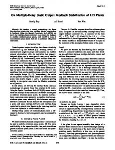
Example 4.2. Consider the following discrete-time networked control system: [ ] [ ] [ ] 0.9 0.5 0.3 0 1 x(k + 1) = x(k) + x(k − d(k)) + u(k) 0.8 0.1 0.8 0.5 0.5 [ ] [ ] 1 1 1 0 y(k) = x(k) + x(k − d(k)) 0 1 1 1 A. Static output feedback stabilization for NCSs without quantisers. In this part, we consider that there are no quantisers in system (21). In [16], the system described by above example can be stabilized by SOF controller (4) for 3 ≤ d(k) ≤ 11 and result in [19] is 3 ≤ d(k) ≤ 12. Under the same SOF controller F = [−0.3550 − 0.1842] in [16], the system is asymptotically stable for dm ≤ d(k) ≤ dM (dm = 3, dM = 13) by using Corollary 3.1. It shows our results are less conservative than [16,19]. B. Static output feedback stabilization for NCSs with quantisers. In this subsection, we consider another case that there is data quantized in the sensor to controller and controller to actuator. The quantisers f (·) and g(·) in (8) and (9) are chosen as logarithmic with ρf = 0.9 and ρg = 0.8 where ∆fi and ∆gj are with entries δf and δg respectively. When the network induced delay satisfying (3) are given by dm = 3, dM = 13 and initial state x0 is given by [2, 1.5]T , by using modified CCL algorithm, we can obtain quantized SOF controller: F = [−0.3037 − 0.1572]. Figure 2 shows the state response of the quantized NCS (21) under the obtained SOF controller.

5. Conclusions. This paper investigated the static output feedback control for discretetime networked control systems with the output and control input signals quantization. The SOF stabilization conditions of quantized discrete-time NCSs have been presented by using the Lyapunov functional approach and introducing relaxation variables technique. Based on these conditions, new stability and stabilization conditions for discrete-time NCSs without quantisers have been proposed. It is worth pointing out that the stability conditions for the systems which have been shown both theoretically and through numerical examples to be less conservative than the existing results. Meanwhile, quantized SOF controller of the NCSs can be solved by using modified CCL algorithm. Numerical examples have shown the effectiveness of the proposed method.

730

Y. LIU AND G. YANG

2.5 x1 x2 2

state response

1.5

1

0.5

0

−0.5

−1

0

10

20

30 time, k

40

50

60

Figure 2. State response of closed-loop NCS with quantisers in Example 4.2 Acknowledgment. This work was supported in part by the Funds for Creative Research Groups of China (No. 60821063), National 973 Program of China(Grant No. 2009CB320604), the Funds of National Science of China(Grant No. 60974043), and the 111 Project (B08015), the Fundamental Research Funds for the Central Universities (No. N090604001, N090604002). REFERENCES [1] B. Zhang, S. Xu and Y. Zou, Improved stability criterion and its applications in delayed controller design for discrete-time systems, Automatica, vol.44, pp.2963-2967, 2008. [2] C. Peng and Y. Tian, Networked H∞ control of linear systems with state quantization, Information Sciences, vol.177, pp.5763-5774, 2007. [3] D. Yue, C. Peng and G. Tang, Guaranteed cost control of linear systems over networks with state and input quantisations, Control Theory and Applications, vol.153, no.6, pp.658-664, 2006. [4] D. Liberzon, Hybrid feedback stabilization of systems with quantized signals, Automatica, vol.39, pp.1543-1554, 2003. [5] E. Tian, D. Yue and X. Zhao, Quantised control design for networked control systems, Control Theory Applications, vol.1, no.6, pp.1693-1699, 2007. [6] F. Fagnani and S. Zampieri, Stability analysis and synthesis for scalar linear systems with a quantized feedback, IEEE Transactions on Automatic Control, vol.48, no.8, pp.1569-1584, 2003. [7] N. Elia and S. Mitter, Stabilization of linear systems with limited information, IEEE Transactions on Automatic Control, vol.46, no.9, pp.1384-1400, 2001. [8] E. Fridman and U. Shaked, An improved stabilization method for linear systems with time-delay, IEEE Transactions on Automatic Control, vol.47, no.11, pp.1931-1937, 2002. [9] E. Fridman and U. Shaked, Stability and guaranteed cost control of uncertain discrete delay systems, International Journal of Control, vol.78, no.4, pp.235-246, 2005. [10] M. Fu and L. Xie, The sector bound approach to quantized feedback control, IEEE Transactions on Automatic Control, vol.50, no.11, pp.1698-1711, 2005. [11] G. Zhai, Y. Mi, I. Joe and K. Tomoaki, Design of H∞ feedback control systems with quantized signals, Proc. of the 16th IFAC World Congress, Prague, pp.1915-1920, 2005. [12] H. Ishii and T. Basar, Remote control of LTI systems over networks with state quantization, Systems and Control Letters, vol.54, pp.15-31, 2005. [13] G. Zhai, X. Chen, J. Imae and T. Kobayashi, Analysis and design of H∞ feedback control systems with two quantized signals, Proc. of 2006 IEEE International Conference on Networking, Sensing and Control, Lauderdale, FL, pp.346-350, 2006.

QUANTIZED SOF STABILIZATION OF DISCRETE-TIME NCSS

731

[14] L. Ghaoui, F. Oustry and M. A. Rami, A cone complementarity linearization algorithm for static output-feedback and related problems, IEEE Transactions on Automatic Control, vol.42, pp.11711176, 1997. [15] S. Azuma and T. Sugie, Optimal dynamic quantizers for discrete-valued input control, Automatica, vol.44, pp.396-406, 2008. [16] H. Gao, C. Wang and Y. Wang, Delay-dependent output-feedback stabilisation of discrete-time systems with time-varying state delay, Control Theory and Applications, vol.151, no.6, pp.691-698, 2004. [17] H. Gao and T. Chen, New results on stability of discrete-time systems with time-varying state delay, IEEE Transactions on Automatic Control, vol.52, no.2, pp.328-333, 2007. [18] R. Brockett and D. Liberzon, Quantized feedback stabilization of linear systems, IEEE Transactions on Automatic Control, vol.45, no.7, pp.1279-1289, 2000. [19] Y. He, G. Liu and J. She, Output feedback stabilization for a discrete-time system with a timevarying delay, IEEE Transactions on Automatic Control, vol.53, no.10, pp.2372-2377, 2008. [20] Y. Moon, P. Park, W. Kwon and Y. Lee, Delay-dependent robust stabilization of uncertain statedelayed systems, International Journal of Control, vol.74, pp.1447-1455, 2001. [21] M. Corradini and G. Orlando, Robust quantized feedback stabilization of linear systems, Automatica, vol.44, pp.2458-2462, 2008. [22] J. Delvenne, An optimal quantized feedback strategy for scalar linear systems, IEEE Transactions on Automatic Control, vol.51, no.2, pp.298-303, 2006. [23] D. Liberzon and D. Nesic, Input-to-state stabilization of linear systems with quantized feedback, IEEE Conference on Decision and Control, Seville, Spain, pp.8197-8202, 2005. [24] X. Zhu and G. Yang, Jensen inequality approach to stability analysis of discrete-time systems with time-varying delay, Proc. of 2008 American Control Conference, Washington, pp.1644-1649, 2008. [25] X. Jiang, Q. Han and X. Yu, Stability criteria for linear discrete-time systems with interval-like time-varying delay, Proc. of 2005 American Control Conference, Portland, OR, pp.2817-2822, 2005. [26] X. Zhu, C. Hua and S. Wang, State feedback controller design of networked control systems with time delay in the plant, International Journal of Innovative Computing, Information and Control, vol.4, no.2, pp.283-290, 2008. [27] Y.-B. Zhao, G.-P. Liu and D. Rees, A predictive control based approach to networked wiener systems, International Journal of Innovative Computing, Information and Control, vol.4, no.11, pp.2793-2802, 2008.