Robust Static Output Feedback Fuzzy Control ... - Semantic Scholar

International Journal of Fuzzy Systems, Vol. 14, No. 1, March 2012

131

Robust Static Output Feedback Fuzzy Control Design for Nonlinear Discrete-Time Systems with Persistent Bounded Disturbances Hwa-Lu Jhi and Chung-Shi Tseng Abstract1

feedback. When dealing with output feedback control design, either a static output feedback case or a dynamic To date, nonlinear l∞ -gain static output feedback output feedback (fuzzy observer-based) case is considcontrol problems have not been solved by the conven- ered [1, 4, 13, 21]. For the dynamic output feedback case, tional control methods for nonlinear discrete-time a fuzzy observer is also involved as well as the fuzzy systems with persistent bounded disturbances. This controller. In other words, for the fuzzy observer-based study introduces static output feedback fuzzy control output feedback control design, a fuzzy observer should also be involved to estimate the system states using the scheme to deal with the nonlinear l∞ -gain control output information and a fuzzy controller is constructed problem. The structure of static output feedback using the estimated states. For the static output feedback fuzzy control is simpler than that of dynamic output case [3, 5, 8, 11, 14, 15, 16, 17, 23], the fuzzy controller feedback fuzzy control. Based on the Takagi and depends on the system outputs only without the complex Sugeno (T-S) fuzzy model, a static output feedback structures of the fuzzy observer. Strictly speaking, some fuzzy controller is developed to minimize the upper of these studies are not purely static output feedback bound of l∞ -gain of the closed-loop system under control cases since their proposed fuzzy controllers still some linear matrix inequality (LMI) constraints. A depend on some measurable states to construct the singular value decomposition (SVD) method is pro- premise variables [8, 16]. In general, the control design posed in this study to solve the l∞ -gain static output of static output feedback is more straightforward but less flexible than that of dynamic output feedback and the feedback fuzzy control problem for the nonlinear dis- structure of static output feedback controller is much crete-time systems in terms of solving an LMI-based simpler than that of dynamic output feedback controller. minimization problem. The proposed static output Unlike the Η ∞ ( l2 -gain) control case [1, 4, 10, 14, 16, feedback fuzzy control scheme can efficiently attenuate the peak of perturbation due to persistent 17, 23, 24], which reduces the influence of the energy of bounded disturbances for the nonlinear discrete-time external disturbance on the energy of output signal as systems. Simulation examples are given to illustrate small as possible, in this study an l∞ -gain static output the design procedures and to confirm the l∞ -gain feedback fuzzy controller is proposed to reduce the influence of the peak (i.e., l∞ -norm) of external disturperformance of the proposed method. Keywords: l∞ -gain control, nonlinear discrete-time systems, static output feedback fuzzy controller, persistent bounded disturbances, LMI constraints.

1. Introduction Recently, there are many successful applications in output feedback fuzzy control using T-S fuzzy model for the nonlinear discrete-time systems [4, 6, 10, 21, 24]. The output feedback control is very important and must be used when the system states are not available for Corresponding Author: Hwa-Lu Jhi is with the Department of Electrical Engineering, Ming Hsin University of Science and Technology, Hsin-Feng 30401, Taiwan. E-mail: [email protected]

bance on the peak (i.e., l∞ -norm) of the output signal as small as possible [22]. Therefore, the l∞ -gain static output feedback fuzzy controller may be more suitable for some practical applications because control engineers may concern more about the peak (amplitude) than the total energy of the perturbed signal. At present, there are no efficient algorithms to solve the l∞ -gain static output feedback control problem for the nonlinear discrete-time systems. Therefore, it is more appealing to develop a feasible method to solve the l∞ -gain static output feedback robust control design for the nonlinear discrete-time systems with persistent bounded disturbances. In this study, first, the T-S fuzzy model is used to represent a nonlinear discrete-time system, then an l∞ -gain performance for the discrete-time system is formulated,

© 2012 TFSA

International Journal of Fuzzy Systems, Vol. 14, No. 1, March 2012

132

and finally an l∞ -gain static output feedback fuzzy controller is developed to reduce the perturbation of states against persistent bounded disturbances as small as possible. The external disturbances in the l2 -gain control design should be with finite energy or bounded l2 -norm but the external disturbances in the l∞ -gain control design should be with finite amplitude or bounded l∞ -norm. From the practical point of view, the sense of amplitude may be more intuitive than that of statistical property or energy. A SVD method is proposed in this study to solve the l∞ -gain static output feedback fuzzy control design for nonlinear discrete-time systems, which can be characterized in terms of solving a linear matrix inequality problem (LMIP) if some scalars are specified in advance. The LMIP can be efficiently solved by using a LMI-based optimization method. The proposed SVD approach provides different aspect from the linear transformation approach [17]. Therefore, our approach does not require any coordination transformation and moreover the proposed SVD method is very simple and easy to follow. The main contributions of this paper are stated as follows: (1). The l∞ -gain static output feedback fuzzy control problem for nonlinear discrete-time systems is studied for the first time. (2). A SVD method is proposed to solve the l∞ -gain static output feedback fuzzy control problem for the nonlinear discrete-time systems in terms of solving an LMI-based minimization problem and the static output feedback fuzzy control gains can be obtained efficiently. (3). Both stability and l∞ -gain disturbance rejection performance are guaranteed for the discrete-time nonlinear control systems. The paper is organized as follows: some notations and definitions are given in Section 2. In Section 3, l∞ -gain static output feedback fuzzy control design for nonlinear discrete-time systems with persistent bounded disturbances is introduced, while some simulation results are presented in Section 4. Finally, concluding remarks are made in Section 5. Some notations and definitions are stated below: T ∗ ⎤ ⎡ M 11 M 21 ⎤ ⎡ M 11 Δ ⎢ ⎥. ⎢M ⎥ ⎣ 21 M 22 ⎦ ⎣ M 21 M 22 ⎦

Δ

x(k )

x(k )

∞

x(k )

x T ( k ) x ( k ) for x ( k ) ∈ R n .

Δ s u p x(k) k

for x ( k ) ∈ R n .

∈ l∞ if x(k )

∞

0 . Note that, since U and V are orthogonal matrices, U T = U −1 ,

V T = V −1 , and then

V T V = VV T = V −1V = VV −1 = I [n×n ] . The final defuzzification outputs of the fuzzy system are inferred as follows: L

∑ μ ( z (k ))( A x(k ) + B u (k ) + B ω (k )) i

i =1

i

1i

2i

L

∑ μ ( z (k ))

(3)

i

i =1

L

= ∑ hi ( z (k )) [ ( Ai x(k ) + B1i u (k ) + B2iω (k ) ] i =1

where g

μi ( z (k )) = ∏ Fij ( z j (k )), hi ( z (k )) = j =1

[

z ( k ) = z1 ( k ),

μi ( z (k )) L

L

L

∑ h ( z(k ))∑ h ( z(k ))[A x(k ) + B i

j

i =1

ij

2i

ω ( k )]

(8)

j =1

where Aij = Ai + B1i K j C for all i, j = 1,2,

, L.

The optimal l∞ -gain fuzzy control problem is to specify the control input u(k ) in (7) such that the following minimax problem is achieved for the nonlinear discrete-time systems in (8) [9, 18]. x(k ) ∞ min sup (9) u ( k ) ω ( k )∈l ω(k ) ∞ ∞ However, it is very difficult to solve the minimax problem in (9) for the nonlinear discrete-time system in (8) directly, the suboptimal approach via minimizing the upper bound of the l∞ -gain is proposed in this study. Let us consider the l∞ -gain performance as follows:

(4)

∑ μi ( z (k ))

The l∞ -gain control problem is said to be solved if there exists a control law u (k ) in (7) such that the following

i =1

]

x ( k + 1) =

,

r ×r

x(k + 1) =

133

, z g ( k ) , and Fij ( z j ( k )) is the grade of

l∞ -gain performance with x (0) = 0 x(k )

membership of z j ( k ) in Fij .

ω(k )

It is assumed that L

≤ ρ , ∀ω ( k ) ∈ l∞

∞

(10)

∞

where ρ is a disturbance attenuation level or

μi ( z (k )) ≥ 0 and ∑ μi ( z (k )) > 0

x(k )

i =1

for all k . Therefore we get

∞

≤ ρ ω (k )

∞,

∀ω ( k ) ∈ l∞

(11)

can be achieved.

hi ( z (k )) ≥ 0 and

Remark 5: If we can make

L

∑ h ( z (k )) = 1. i =1

i

(5)

Suppose the following static output feedback fuzzy controller is proposed to deal with the nonlinear discrete-time system (1). Control Rule j: If z1 ( k ) is F j1 and z g ( k ) is F jg (6) Then u( k ) = K j y ( k )

x( k )

ω(k )

∞

≤ ρ , then the

peak of

∞

the state x (k ) can be attenuated by a level ρ under the effect of the peak of the persistently bounded input signal ω (k ) . If the initial condition is considered, i.e., x (0) ≠ 0, the l∞ -gain in (11) is modified as follows x(k )

∞

≤ β x ( 0) + ρ ω ( k )

∞

(12)

where K j is the static output feedback fuzzy control

where β and ρ are some positive scalars.

gain for the J th control rule. Hence, the overall static output feedback fuzzy controller is proposed as

Remark 6: The l∞ -gain performance in (11) is equivalent to the bounded input bound (error) state stability (Moreover, the l∞ -gain performance in (12) is called

u( k ) =

L

∑ h ( z(k )) K j

j y ( k ).

(7)

j =1

Remark 4: Note that the proposed static output feedback fuzzy controller depends on the system output y(k) only. The structure of the static output feedback fuzzy controller is very simple and easy to be implemented. After manipulation, the closed-loop nonlinear system

l∞ -stable with finite gain). The purpose of this study is to determine a fuzzy controller in (7) for the closed-loop system in (8) with the guaranteed l∞ -gain performance in (12) for all

ω (k) ∈ l∞ . Thereafter, the attenuation level ρ can be minimized so that the l∞ -gain performance in (12) is

International Journal of Fuzzy Systems, Vol. 14, No. 1, March 2012

134

reduced as small as possible at steady-state. First, one useful lemma is stated below. Lemma 1: If a real scalar function ω ( k ) satisfies the following difference inequality ω ( k + 1) ≤ ςω ( k ) + συ ( k ) (13) where 0 ≤ ς < 1 and σ > 0 , then k −1

ω ( k ) ≤ ς k ω (0) + σ ∑ ς rυ ( k − r − 1).

L 1 L = {∑hi ( z(k ))∑hj ( z(k ))[( Aij + Aji ) x(k ) + 2Biω(k )]}T 4 i=1 j =1 L

r =1

−

−

[

+ 2B2iω(k )]T P [( Aij + Aji ) x(k ) + 2B2iω(k )]}

hold for

i ≤ j (i, j = 1,2, −1

B2 i

, L)

s.t.

⎤ ∗ ⎥ ∗ ⎥ < 0 (15) ⎥ − Q⎥ ⎦⎥

hi (⋅) ∩ h j (⋅) ≠ φ

where Ai = V AiV , B1i = V B1i , B2i = V −1 B2i , then l∞ − gain control performance in (12) is guaranteed for an

−1

attenuated

level

ρ=

L

Aij + Aji

i =1

j =1

2

+ B2iω(k )]T P [( =

Aij + Aji 2

∑

c (1 − α )λ min ( P )

,

∑

+ αx T ( k ) Px ( k ) + cω ( k ) T ω ( k )

where 0 ≤ α < 1 and c are positive scalars. If ⎡ Aij + A ji T Aij + A ji ⎤ ∗ ) P( ) −α P ⎢( ⎥ 2 2 ⎢ ⎥ < 0 (16) Aij + A ji T T ⎢ B2 i P ( B2i PB2i − cI ⎥ ) 2 ⎣⎢ ⎦⎥ for all i ≤ j (i, j = 1,2, , L), we obtain 1 P 2 x(k

2

+ 1) ≤ αx T (k ) Px(k ) + cω T (k )ω(k )

(17)

Proof: For a symmetric positive definite matrix P , from (8) we obtain

+ c ω ( k − τ − 1)

2

= {∑ hi ( z (k ))∑ h j ( z (k ))[ Aij x(k ) + B2iω (k )]}

m =1

2

2

2

≤α k P 1 / 2 x (0) + c

k −1

α τ ω ( k − τ − 1) ∑ τ

{

≤ sup α k P 1 / 2 x (0)

2

k −1

α τ }= sup {α ∑ τ [ ] τ ∈ 0, k −1

=0

k

2

τ ∈[0, k −1]

=0

2

2

P 1 / 2 x (0) +

From above, we have λ min ( P ) x ( k ) ≤ 2

2 1 2 P x(k )

L

× P{∑ hr ( z (k ))∑ hm ( z (k ))[ Arm x(k ) + B2 rω (k )]} r =1

P 1 / 2 x(k )

T

j =1

L

1

= α P 2 x(k ) + c ω(k )

1−αk c ω ( k − τ − 1) ( )}. 1−α

P x(k + 1) = x (k + 1) Px(k + 1)

i =1

2

2

T

L

T

⎡ Aij + A ji T Aij + A ji ⎤ ∗ ) P( ) −αP ⎢( ⎥ ⎡ x(k ) ⎤ 2 2 ×⎢ ⎥⎢ + A A ω ( k )⎥⎦ ij ji ⎢ B 2Ti P ( ) B2Ti PB2i − cI ⎥ ⎣ 2 ⎣⎢ ⎦⎥

By Lemma 1, we obtain

L

) x(k ) + B2iω(k )]}

⎡ Aij + A ji T Aij + A ji ⎤ T ∗ ) P( ) −αP ⎥ ⎡ x ( k ) ⎤ ⎢( 2 2 hi2 ( z ( k )) ⎢ ⎥ ⎥ ⎢ + A A ( ) ω k ij ji T T ⎣ ⎦ ⎢ i =1 B2i P( ) B 2i PB 2i − cI ⎥ 2 ⎣⎢ ⎦⎥

λ (P ) and β = max , where λmax ( P ) and λmin ( P ) λmin ( P ) denote the maximal and minimal eigenvalues of P = (V −1 )T Q −1 (V −1 ) = VQ −1V T , respectively, and the steady fuzzy control gain can be obtained as K j = Y j Q1−1 ∑ −1 U −1 ,

1 2

) x(k )

L

∑

]

∗ − cI

L

= {∑hi ( z(k ))∑hj ( z(k ))[(

L L ⎡ x(k ) ⎤ ⎡ x(k ) ⎤ ×⎢ h j ( z ( k )) ⎢ ⎥ + 2 hi ( z ( k )) ⎥ ω ( k ) ⎣ ⎦ ⎣ω ( k )⎦ i =1 j =1, j < i

Y j = Y j [m×r ] 0[m×( n −r ) ] ∈ R m×n such that the following matrix inequalities ⎡ − αQ ⎢ ⎢ 0 ⎢(A Q + B Y ) + (A Q + B Y ) 1i j j 1j i ⎢ i 2 ⎣⎢

L

1 ≤ {∑hi ( z(k ))∑hj ( z(k ))[( Aij + Aji ) x(k ) 4 i=1 j =1

(14)

and matrices Y j with

m=1

L

r =0

Proof: The proof is trivial. Then, we obtain the following main result: Theorem 1: In the nonlinear system (8), if there exist two positive scalars 0 ≤ α < 1 and c, a symmetric positive definite matrix Q with 0 ⎡Q1[r×r ] ⎤ n ×n Q=⎢ ⎥∈R , 0 Q 2 [( n − r )×( n − r ) ] ⎦ ⎣

L

× P{∑hr ( z(k ))∑hm ( z(k ))[( Arm + Amr ) x(k ) + 2B2rω(k )]}

≤ sup {α

k

τ ∈[ 0,k −1]

+ c ω ( k − τ − 1) ( 2

2 1 2 P x ( 0)

(18)

1−α )}. 1−α k

Performing “ sup ” to both sides of the above inek∈[0,∞ )

H.-L. Jhi et al.: Robust Static Output Feedback Fuzzy Control Design for Nonlinear Discrete-Time Systems

⎡ − αP ∗ ⎢ ⎢ 0 − cI ⎢ Aij + A ji ) P B2i ⎢P ( 2 ⎣

quality, we obtain

sup λmin ( P ) x(k )

2

k ∈[ 0, ∞ )

≤ sup sup {α k P1/2 x(0)

2

k∈[ 0, ∞ ) τ ∈[0, k −1]

(19)

1−α k )} + c ω (k − τ − 1) ( 1−α 2 c 2 sup ω (k ) . ≤ P1/2 x(0) + 1 − α k∈[0,∞ ) 2

The above inequality implies that

λmin ( P ) x(k )

2 ∞

c 2 ω (k ) ∞ 1−α c 2 2 ω (k ) ∞ . ≤ λmax ( P ) x(0) + 1−α 2

≤ P1/2 x(0) +

(20)

x(k ) ≤

2 ∞

λmax ( P ) c 2 x(0) + ω (k ) λmin ( P ) (1 − α ) λmin ( P ) λmax ( P ) x(0) λmin ( P )

≤(

c ω (k ) ∞ )2 . (1 − α )λmin ( P )

+ or

x(k )

∞

λmax ( P ) x(0) λmin ( P )

≤ +

c ω (k ) (1 − α )λmin ( P )

0 0⎤ I 0⎥ ⎥ 0 V ⎥⎦

T

and post-multiplying

0 0⎤ I 0 ⎥ to (26), we obtain ⎥ 0 V ⎥⎦ ⎡ − αP ∗ ⎢ ⎢ − cI 0 ⎢ Aij + A ji ⎢ P( ) P B 2i 2 ⎣

⎤ ∗ ⎥ ∗ ⎥ < 0, ⎥ − P⎥ ⎦

(27)

where Aij = (V −1 ) AijV

(21)

B2i = (V −1 ) B2i .

∞

for all ω ( k ) ∈ l∞ . Note that (16) is equivalent to T ⎡ Aij + A ji ⎤ ⎡ Aij + A ji ⎤ ( ) B ) B2i ⎥ 2 i ⎥ P ⎢( ⎢ 2 2 ⎣ ⎦ ⎣ ⎦

⎡ − αP 0 ⎤ +⎢ ⎥ < 0. − cI ⎦ ⎣ 0 Obviously, (22) is equivalent to

By

(22)

⎡Q ⎢0 ⎢ ⎢⎣ 0

⎡Q 0 0 ⎤ pre-multiplying ⎢ 0 I 0 ⎥ and post-multiplying ⎢ ⎥ ⎢⎣ 0 0 Q ⎥⎦ 0 0⎤ I 0 ⎥ to (27), we obtain ⎥ 0 Q ⎥⎦ ⎡ − αQ ∗ ⎢ ⎢ − cI 0 ⎢ Aij + A ji ⎢( )Q B 2i 2 ⎣

T

⎤ ⎡ Aij + A ji ⎤ ⎡ Aij + A ji ) P B2i ⎥ P −1 ⎢ P ( ) P B2i ⎥ ⎢P ( 2 2 ⎦ ⎣ ⎦ ⎣ ⎡ − αP +⎢ ⎣ 0

(24)

P = (V −1 )T P (V −1 ) (25) where P is a symmetric positive definite matrix then (24) is rewritten as ⎡ − α (V −1 )T P (V −1 ) ⎤ ∗ ∗ ⎢ ⎥ − cI ∗ 0 ⎢ ⎥ < 0, (26) − 1 T − 1 ⎢ M 31 M 32 − (V ) P (V )⎥⎦ ⎣ Aij + A ji where M 31 = (V −1 )T P (V −1 )( ) 2 and M 32 = (V −1 )T P (V −1 ) B2i .

⎡V ⎢0 ⎢ ⎢⎣ 0

2 ∞

⎤ ∗ ⎥ ∗ ⎥ < 0. ⎥ − P⎥ ⎦

Let

⎡V By pre-multiplying ⎢ 0 ⎢ ⎢⎣ 0

Hence,

135

(23)

0 ⎤ ⎥ < 0. − cI ⎦

By the Schur complements [2], (23) is equivalent to the following matrix inequalities

where Q = P −1 . By observing that

⎤ ∗ ⎥ ∗ ⎥ < 0, ⎥ − Q⎥ ⎦

(28)

International Journal of Fuzzy Systems, Vol. 14, No. 1, March 2012

136

(

[ Ai + B1i K jUSV −1 ] [ A j + B1 j K iUSV −1 ] Aij + A ji ) = (V −1 ){ }V + 2 2 2 −1 −1 −1 −1 [V AiV + V B1i K jUS ] [V A jV + V B1 j K iUS ] } ={ + 2 2 Ai + B 1i K jUS ] [ A j + B 1 j K iUS ] } ={ + 2 2

(29)

where Ai = V −1 AiV and B1i = V −1 B1i , then (28) can be expressed as ⎤ ∗ ⎥ ∗ ⎥ 0 , and

(34) (15). T Since Q = Q > 0 is the variable to be solved in (34), c should be modithe term (1 − α )λmin [(V −1 ) T Q −1 (V −1 )] fied as follows to solve the minimization problem in (34). Note that

(36)

Since Q and V T V = I . By pre-multiplying post-multiplying Q to (36), we obtain c QQ − ε 2Q < 0 (37) (1 − α ) which is equivalent to ⎡ − ε 2Q ⎤ Q ⎢ (38) (1 − α ) ⎥ < 0 − I⎥ ⎢ Q c ⎣ ⎦ by the usage of the Schur complements [2]. Finally, the minimization problem in (34) can be reformulated as follows: min ε 2 subject to

(33)

control gain can also be obtained as K j = Y j Q1−1 ∑ −1 U −1 .

(35)

Consequently, x ( k ) ∞ ≤ β x ( 0) + ρ ω ( k )

∞

(39)

< β x ( 0) + ε ω ( k ) ∞ .

According to the analysis above, the static output feedback l∞ − gain control problem via fuzzy control scheme is summarized as follows: Design Procedure: Step 1: Construct the fuzzy plant rules in (1). Step 2: Given a set of 0 ≤ α < 1 and c > 0 . Step 3: Given an initial ε 2 . Step 4: Solve the following linear matrix inequality problem (LMIP) ⎡ ⎢ − αQ ∗ ⎢ cI − 0 ⎢ ⎢ ⎧⎪ ( Ai Q + B1i Y j ) + ( A j Q + B1 j Yi ) ⎫⎪ ⎢⎨ ⎬ B2 i 2 ⎪⎭ ⎣⎢ ⎪⎩

and

⎤ ∗ ⎥ ⎥ ∗ ⎥ 0 can not be found. If Q > 0 can not be found for all possible ε 2 , try another set of 0 ≤ α < 1 and 0 < c and repeat Step 3-5. Step 6: Construct the static output feedback fuzzy controller (7). Remark 7: Note that (40) is a standard LMIP, if 0 < ε 2 , 0 ≤ α < 1, and 0 < c are given in advance. ThereQ = diag{Q1 ,Q2 } and fore, parameters K j = Y j Q1−1 ∑ −1 U −1 can be determined simultaneously from (40). Software packages such as LMI optimization toolbox in Matlab [12] have been developed for this purpose and can be employed to easily solve the LMIP. Remark 8: The above Design Procedure can be made simpler by letting c = (1 − α ) (or α = 1 − c ) then the minimization problem in (39) can be solved by performing one-dimensional search on the parameter 0 ≤ α < 1 .

and

⎡0.1⎤ B21 = B22 = ⎢ ⎥, ⎣0.1⎦

1 y (k ) ) = h1 ( y (k )), F1 ( y (k )) = (1 − κ 2 1 y (k ) ) = h2 ( y (k )), and κ = 30 . F2 ( y (k )) = (1 + κ 2

Then the SVD of C is given as follows: T ⎡1 0 ⎤ C = [1 0] = [1][1 0] ⎢ ⎥ . ⎣0 1 ⎦ As mentioned in Remark 8, the Design Procedure in the above section can be made simpler by letting c = (1 − α ) (or α = 1 − c ) then the minimization problem in (39) can be solved by performing one-dimensional search on the parameter 0 ≤ α < 1 . According to the Design Procedure, the following table shows subminimal values of ε 2 corresponding to some values of α .

α ε2 α ε2

3. Simulation Examples Example 1: To illustrate the proposed fuzzy control approach, a control problem of stabilizing a discrete-time chaotic system is considered in this study. For this example, the Henon Mapping Model with additional input and output terms is given by

Y 2 = [Y2

y ( k ) = x1 ( k )

where external disturbance ω (k ) = 1.0sin( πk ) ∈ l ∞.

ρ=

10

The Henon Mapping Model can be exactly represented by the following two-rule fuzzy model under x1 (k ) (= y (k )) ∈[ −κ κ ] [20].

where x ( k ) = [x1 ( k ), x2 ( k )] , u( k ) = 1.4 + u ( k ), T

∗

and

and

0.4 (0.3873) 2 0.95 (0.7616) 2

0.5 (0.3317) 2 0.99 (1.4142) 2

0 ⎤ ⎡0.0446 Q=⎢ , Y 1 = [Y1 0] = [− 1.3468 0], 0.1098⎥⎦ ⎣ 0

(41)

Rule 1: IF y (k ) is F1 THEN x ( k + 1) = A1 x( k ) + B11u( k ) + B21ω ( k ), y ( k ) = Cx ( k ). Rule 2: IF y (k ) is F2 THEN x ( k + 1) = A2 x ( k ) + B12 u( k ) + B22ω ( k ), y ( k ) = Cx ( k ).

0.302 ( 2.1679) 2 0.7 (0.3606) 2

In the case of α = 1 − c = 0.5 and ε = 0.3317, the LMIP in (40) is solved using the LMI optimization toolbox in Matlab as follows.

x1 ( k + 1) = − x12 ( k ) + 0.3 x 2 ( k ) + 1.4 + u ∗ ( k ) + 0.1ω ( k ) x 2 ( k + 1) = x1 ( k ) + 0.1ω ( k )

137

0] = [1.327 0],

c = 0.3314, (1 − α )λmin [(V −1 ) T Q −1 (V −1 )]

and β=

λ max [(V −1 ) T Q −1 (V −1 )] 22.4396 = = 1.5699 −1 T −1 −1 9.1043 λ min [(V ) Q (V )]

The static output feedback fuzzy control gains are found to be K1 = [ −30.2227], K 2 = [29.7773] . Hence, the static output feedback fuzzy controller is constructed as follows u( k ) =

2

∑ h ( y(k )) K j

j

y(k ) .

j =1

The ratio of the peak of x (k ) to the peak of ω (k ) for k ≥ 80 in this example is

International Journal of Fuzzy Systems, Vol. 14, No. 1, March 2012

138

x(k )

ω (k )

∞ ∞

=

1 y (k ) − 6 ) = h2 ( y1 (k )). F2 ( y1 (k )) = (1 + 1 2 14 The SVD of C is given as follows:

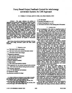
0.2604 = 0.2604 < ρ = 0.3314. 1 .0

The trajectories of x1 and x2 are shown in Fig. 1(a). T 1 0 ⎤ ⎡ 0 The control signal is applied at k = 20 and shown in ⎡1 0 0⎤ ⎡0 1⎤ ⎡5.099 0 0⎤ ⎢ ⎥ C=⎢ ⎥ = ⎢1 0⎥ ⎢ 0 ⎥ ⎢0.9806 0 − 0.1961⎥ Fig. 1(b). From Fig. 1(a), one observes that the states are 0 5 1 1 0 ⎣ ⎦ ⎣ ⎦⎣ ⎦ ⎢ 0.1961 0 0.9806 ⎥ ⎣ ⎦ very oscillating before k < 20 but all states are stabiSimilarly, the Design Procedure in the above section lized rapidly after the control signal is applied. From these simulation results, the proposed static output feed- can be made simpler by letting c = (1 − α ) or back fuzzy control clearly results in a desired l∞ − gain ( α = 1 − c ) then the minimization problem in (39) can be solved by performing one-dimensional search on the paperformance. rameter 0 ≤ α < 1 . According to the Design Procedure, 2 the following table shows subminimal values of ε 2 corx1 1 x2 responding to some values of α . 0 -1 -2

0

20

40 60 (a) time sequence k

80

100

0

0.9

0.915 2

(0.9695) 0.95

(0.9747) 2

(0.995) 2

(1.0954) 0.945

0.925 2

(0.94604) 2 0.99 (1.9235) 2

control input

-0.5

-1

-1.5

α ε2 α ε2

0

20

40 60 (b) time sequence k

80

100

Fig. 1 (a) The trajectories of x1 ( k ) and x 2 ( k ) . (b) The control signal u * ( k ) .

Example 2: Consider the following two-rule T-S fuzzy model [4]: Rule 1: IF y1 ( k ) is about F1 THEN x ( k + 1) = A1 x ( k ) + B11u( k ) + B21ω ( k ), and y ( k ) = Cx( k ). Rule 2: IF y1 ( k ) is about F2 THEN x ( k + 1) = A2 x ( k ) + B12 u( k ) + B22ω ( k ), and y ( k ) = Cx( k ). where T T x ( k ) = [x1 ( k ), x2 ( k ), x3 ( k )] , y ( k ) = [ y1 ( k ), y 2 ( k )] ,

πk ⎤ ⎡ and ω ( k ) = 5 sign ⎢sin( )⎥ is a periodic square wave. 10 ⎦ ⎣ 0.89 0.5⎤ ⎡ 0 ⎡ 0 ⎢ ⎥ A1 = ⎢ −0.6 0.89 0 ⎥ , A2 = ⎢⎢ 0.03 ⎢⎣ −0.1 0 ⎢⎣ −0.1 0.9 ⎥⎦ ⎡0⎤ ⎡0.04 ⎤ ⎡1 ⎢ ⎥ B12 = ⎢1 ⎥ , B21 = B22 = ⎢⎢0.04 ⎥⎥ , C = ⎢ ⎣0 ⎢⎣0 ⎥⎦ ⎢⎣0.04 ⎥⎦

0.89 0.5⎤ ⎡1 ⎤ ⎥ 0.89 0 ⎥ , B11 = ⎢⎢0 ⎥⎥ , ⎢⎣1.5⎥⎦ 0 0.9⎥⎦ 0 0⎤ 5 1 ⎥⎦

1 y (k ) − 6 F1 ( y1 (k )) = (1 − 1 ) = h1 ( y1 (k )), 2 14

In the case of α = 1 − c = 0.925 and ε = 0.94604 , the LMIP in (40) is solved using the LMI optimization toolbox in Matlab as follows. 0 ⎤ ⎡0.3191 0.3041 ⎢ 0 ⎥, Q = 0.3041 0.7344 ⎥ ⎢ ⎢⎣ 0 0 0.2687 ⎥⎦

Y 1 = [Y1

0] = [− 0.0183 − 0.0443 0],

Y 2 = [Y 2

ρ=

and β =

0] = [− 0.0233 − 0.0532 0],

c = 0.94603. (1 − α )λ min [(V −1 ) T Q −1 (V −1 )]

λmax [(V −1 ) T Q −1 (V −1 )] 6.3093 = = 2.3763 . −1 T −1 −1 1.1174 λmin [(V ) Q (V )]

The static output feedback fuzzy control gains are found to be K1 = [ − 0.0605 4.572 × 10 −5 ],

K 2 = [− 0.0718 − 0.0003] and hence the static output

feedback fuzzy controller is constructed as follows u( k ) =

2

∑ h ( y (k )) K j

1

j y ( k ).

j =1

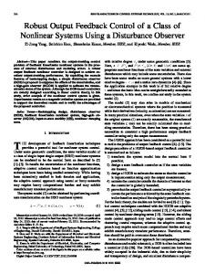
The trajectories of x1 ( k ) , x2 ( k ) , and x3 ( k ) are shown in Fig. 2(a) while the control signal is shown in Fig. 2(b). The ratio of the peak of x (k ) to the peak of ω (k ) for k ≥ 50 in this example is x(k )

ω(k )

∞ ∞

=

0.9098 = 0.182 < ρ = 0.94603 . 5

H.-L. Jhi et al.: Robust Static Output Feedback Fuzzy Control Design for Nonlinear Discrete-Time Systems

20 15

x1

10

x3

[2]

x2

5 0 -5

[3] 0

20

40 60 (a) time sequence k

80

100

0.5 0 -0.5

[4]

control input

-1 -1.5

0

20

40 60 (b) time sequence k

80

100

Fig. 2 (a) The trajectories of x1 ( k ) , x 2 ( k ) , and x3 ( k ) . (b) The control signal u(k ) .

From these simulation results, the proposed static output feedback fuzzy control clearly results in a desired l∞ -gain performance.

[5]

[6]

4. Conclusions In this study, l∞ -gain static output feedback control problem for a nonlinear discrete-time system is solved by the fuzzy control scheme. Based on the T-S fuzzy model, a static output feedback fuzzy controller is developed to reduce the perturbation of states against persistent bounded disturbances by reducing the attenuation level as small as possible. A SVD method is proposed to solve l∞ -gain static output feedback control problem in terms of solving an LMI-based minimization problem. Both stability and l∞ -gain disturbance rejection performance are guaranteed for the static output feedback fuzzy control scheme. Since the peak of the system is a greater concern than statistical property or energy in some design cases, the proposed l∞ -gain static output feedback fuzzy control for nonlinear discrete-time systems is more appealing in some practical applications. Several simulation results have confirmed the elimination of the peak of the output signal against the persistent bounded disturbances for the nonlinear discrete-time system by the proposed l∞ -gain static output feedback fuzzy control scheme.

[7]

[8]

[9]

[10]

[11]

References [1]

C. Peng, L.-Y. Wen, and J.-Q. Yang, “On Delay-dependent Robust Stability Criteria for Uncertain T-S Fuzzy Systems with Interval Time-varying

[12]

[13]

139

Delay,” International Journal of Fuzzy Systems, vol. 13, no. 1, pp. 35-44, March 2011. S. Boyd, L. El Ghaoui, E. Feron, and V. Balakrishnan, Linear Matrix Inequalities in Systems and Control Theory, Philadelphia: SIAM, 1994. Y.-C. Chang, S.-S. Chen, S.-F. Su, and T.-T. Lee, “Static Output Feedback Stabilization for Nonlinear Interval Time-Delay Systems via Fuzzy Control Approach,” Fuzzy Sets and Systems, vol. 148, no. 3, pp.395-410, Dec. 2004. C.-L. Chen, G. Feng, D. Sun, and X.-P. Guan, “ H ∞ Output Feedback Control of Discrete-Time Fuzzy Systems with Application to Chaos Control,” IEEE Trans. Fuzzy Systems, vol. 13, no. 4, pp.531-543, Aug. 2005. S.-S. Chen, Y.-C. Chang, S.-F. Su, S.-L. Chung, and T.-T. Lee, “Robust Static Output-Feedback Stabilization for Nonlinear Discrete-Time Systems with Time Delay via Fuzzy Approach,” IEEE Trans. Fuzzy Systems, vol. 13, no. 2, pp. 263-272, April 2005. T.-S. Chiang, C.-S. Chiu, and P. Liu, “Fuzzy Output Regulation Design of Discrete Affine Systems with Multiple Time-Varying Delays,” Fuzzy Sets and Systems, vol. 160, no. 4, pp. 463-481, Feb. 2009. M. Chilali and P. Gahinet, “ H ∞ design with pole placement constraints: An LMI approach,” IEEE Trans. Automat. Contr., vol.41, no.3, pp.358-367, March 1996. H.-Y. Chung, S.-M. Wu, F.-M. Yu, and W.-J. Chang, “Evolutionary Design of Static Output Feedback Controller for Takagi-Sugeno Fuzzy Systems,” IET-Control Theory & Applications, vol. 1, no. 4, pp.1096-1103, July 2007. M. A. Dahleh and J. B. Pearson, Jr., “ l1 -Optimal Feedback Controllers for MIMO Discrete-Time Systems,” IEEE Trans. Automat. Contr., vol. 32, no. 4, pp. 314-322, April 1987. L.-K. Wang and X.-D. Liu, “Robust H ∞ Fuzzy Output Feedback Control for Uncertain Discrete-time Nonlinear Systems,” International Journal of Fuzzy Systems, vol. 12, no. 3, pp. 218-226, Sep. 2010. C.-H. Fang, Y.-S. Liu, S.-W. Kau, L. Hong, and C.-H. Lee, “A New LMI-Based Approach to Relaxed Quadratic Stabilization of T-S Fuzzy Control Systems,” IEEE Trans. Fuzzy Systems, vol. 14, no. 3, pp. 386-397, June 2006. P. Gahinet, A. Nemirovski, A. J. Laub, and M. Chilali, The LMI Control Toolbox, Natick, MA: The MathWorks, Inc. 1995. T. M. Guerra, A. Kruszewski, L. Vermeiren, and H.

140

[14]

[15]

[16]

[17]

[18]

[19]

[20]

[21]

[22]

[23]

[24]

International Journal of Fuzzy Systems, Vol. 14, No. 1, March 2012

Tirmant, “Conditions of Output Stabilization for Nonlinear Models in the Takagi-Sugeno's Form,” Fuzzy Sets and Systems, vol. 157, no. 9, pp. 1248-1259, May 2006. D. Huang and S. K. Nguang, “Robust H ∞ Static Output Feedback Control of Fuzzy Systems: An ILMI Approach,” IEEE Trans. Systems, Man and Cybernetics, Part B, vol. 36, no. 1, pp. 216-222, Feb. 2006. D. Huang and S. K. Nguang, “Static Output Feedback Controller Design for Fuzzy Systems: An ILMI Approach,” Information Sciences, vol. 177, no. 14, pp. 3005-3015, July 2007. S.-W. Kau, H.-J. Lee, C.-M. Yang, C.-H. Lee, L. Hong, and C.-H. Fang, “Robust H ∞ Fuzzy Static Output Feedback Control of T-S Fuzzy Systems with Parametric Uncertainties,” Fuzzy Sets and Systems, vol. 158, no. 3, pp. 135-146, Jan. 2007. J.-C. Lo and M.-L. Lin, “Robust H ∞ Nonlinear Control via Fuzzy Static Output Feedback,” IEEE Trans. Circuits and Systems-I: Fundamental Theory and Applications, vol. 50, no. 11, pp. 1494-1502, Nov. 2003. J. S. Shamma, “Nonlinear State-Feedback for l1 Optimal Control,” Syst. and Contr. Lett., vol. 21, pp. 265-270, 1993. T. Takagi and M. Sugeno, “Fuzzy Identification of Systems and its Applications to Modeling and Control,” IEEE Trans. Syst., Man, Cybern., vol. 15, pp. 116-132, Jan./Feb. 1985. K. Tanaka and H. O. Wang, Fuzzy Control Systems Design and Analysis: A Linear Matrix Inequality Approach, John Wiley & Sons, Inc. 2001. C.-S. Tseng, “Model Reference Output Feedback Fuzzy Tracking Control Design for Nonlinear Discrete-Time Systems with Time-Delay,” IEEE Trans. Fuzzy Systems, vol. 14, no. 1, pp. 58-70, Feb. 2006. C.-S. Tseng and C.-K. Hwang, “Fuzzy Observer-Based Fuzzy Control Design for Nonlinear Systems with Persistent Bounded Disturbances,” Fuzzy Sets and Systems, vol. 158, no. 2, pp. 164-179, Jan. 2007. H.-N. Wu, “An ILMI Approach to Robust H ∞ Static Output Feedback Fuzzy Control for Uncertain Discrete-Time Nonlinear Systems,” Automatica, vol. 44, no. 9, pp. 2333-2339, Sep. 2008. C.-F. Chuang, W.-J. Wang, Y.-J. Sun, and Y.-J. Chen, “T-S Fuzzy Model Based H ∞ Finite-Time Synchronization Design for Chaotic Systems,” International Journal of Fuzzy Systems, vol. 13, no. 4, pp. 358-368, Dec. 2011.

Hwa-Lu Jhi received his M. S. degree in electrical engineering from Louisiana Tech University in 1984. He was a candidate for Ph.D. at the department of electrical engineering in National Tsing Hua University, Hsinchu, Taiwan. He is currently a lecture in the department of electrical engineering at Ming Hsin University of Science and Technology, Hsin-Feng, Taiwan. His research interests include fuzzy control, digital signal processing, and wireless MIMO communication. Chung-Shi Tseng received the B. S. degree from Department of Electrical Engineering, National Cheng Kung University, Tainan, Taiwan, and the M.S. degree from the Department of Electrical Engineering and Computer Engineering, University of New Mexico, Albuquerque, NM, U.S.A., and the Ph.D. degree in the electrical engineering, National Tsing-Hua University, Hsin-Chu, Taiwan, in 1984, 1987, and 2001, respectively. He is currently a full Professor at Ming Hsin University of Science and Technology, Hsin-Feng, Taiwan. His research interests are in nonlinear robust control, adaptive control, fuzzy control, fuzzy signal processing, and robotics.