P. Facchi and S. Pascazio. Dipartimento di Fisica, Universit`a di Bari I-70126 Bari, Italy and. Istituto Nazionale di Fisica Nucleare, Sezione di Bari, I-70126 Bari, ...
Quantum Zeno subspaces P. Facchi and S. Pascazio Dipartimento di Fisica, Universit` a di Bari I-70126 Bari, Italy and Istituto Nazionale di Fisica Nucleare, Sezione di Bari, I-70126 Bari, Italy (Dated: February 1, 2008) The quantum Zeno effect is recast in terms of an adiabatic theorem when the measurement is described as the dynamical coupling to another quantum system that plays the role of apparatus. A few significant examples are proposed and their practical relevance discussed. We also focus on decoherence-free subspaces.
arXiv:quant-ph/0201115v2 4 Jul 2002
PACS numbers: 03.65.Xp, 03.67.Lx
If very frequent measurements are performed on a quantum system, in order to ascertain whether it is still in its initial state, transitions to other states are hindered and the quantum Zeno effect takes place [1, 2]. This phenomenon stems from general features of the Schr¨odinger equation that yield quadratic behavior of the survival probability at short times [3, 4]. The first realistic test of the quantum Zeno effect (QZE) for oscillating (two-level) systems was proposed about 15 years ago [5]. This led to experiments, discussions and new proposals [6]. A few years ago, the presence of a short-time quadratic region was experimentally confirmed also for a bona fide unstable system [7]. The same experimental setup has been used very recently [8] in order to prove the existence of the Zeno effect (as well as its inverse [9, 10]) for an unstable quantum mechanical system, leading to new ideas [11, 12]. It is important to stress that the quantum Zeno effect does not necessarily freeze everything. On the contrary, for frequent projections onto a multi-dimensional subspace, the system can evolve away from its initial state, although it remains in the subspace defined by the measurement. This continuing time evolution within the projected subspace (“quantum Zeno dynamics”) has been recently investigated [13]. It has peculiar physical and mathematical features and sheds light on some subtle mathematical issues [2, 14, 15]. All the above-mentioned investigations deal with what can be called “pulsed” measurements, according to von Neumann’s projection postulate [16]. However, from a physical point of view, a “measurement” is nothing but an interaction with an external system (another quantum object, or a field, or simply another degree of freedom of the very system investigated), playing the role of apparatus. In this respect, if one is not too demanding in philosophical terms, von Neumann’s postulate can be regarded as a useful shorthand notation, summarizing the final effect of the quantum measurement. This simple observation enables one to reformulate the QZE in terms of a (strong) coupling to an external agent. We emphasize that in such a case the QZE is a consequence of the dynamical features (i.e. the form factors) of the coupling between the system investigated and the external sys-
tem, and no use is made of projection operators (and non-unitary dynamics). The idea of “continuous” measurement in a QZE context has been proposed several times during the last two decades [18, 19], although the first quantitative comparison with the “pulsed” situation is rather recent [20]. The purpose of the present article is to cast the quantum Zeno evolution in terms of an adiabatic theorem and study possible applications. We will see that the evolution of a quantum system is profoundly modified (and can be tailored in an interesting way) by a continuous measurement process: the system is forced to evolve in a set of orthogonal subspaces of the total Hilbert space and a dynamical superselection rule arises in the strong coupling limit. These general ideas will be corroborated by some simple examples. We start by considering the case of “pulsed” observation. We first extend Misra and Sudarshan’s theorem [2] in order to accomodate multiple projectors. Let Q be a quantum system, whose states belong to the Hilbert space H and whose evolution is described by the unitary operator U (t) = exp(−iHt), where H is a time-independent lower-bounded Hamiltonian. Let P {Pn }n (Pn Pm = δmn Pn , n Pn = 1) be a (countable) collection of projection operators and RanPn = HPn the relative subspaces. ThisLinduces a partition on the total Hilbert space H = n HPn . Let ρ0 be the initial density matrix of the system. We “prepare” the system by performing an initial measurement, described by the superoperator X Pˆ ρ = Pn ρPn = ρ0 . (1) n
The free evolution reads ˆt ρ0 = U (t)ρ0 U † (t), U
U (t) = exp(−iHt)
(2)
and the Zeno evolution after N measurements in a time t is governed by the superoperator � �N −1 (N ) ˆ (t/N ) Pˆ Vˆt = Pˆ U , (3) which yields (N ) ρ(t) = Vˆt ρ0 =
X
n1 ,...,nN
)† ) (t), (4) (t) ρ0 Vn(N Vn(N 1 ...nN 1 ...nN
2 where ) (t) = PnN U (t/N ) PnN −1 · · · Pn2 U (t/N ) Pn1 . (5) Vn(N 1 ...nN
We follow [2] and assume for each n the existence of the strong limits (t > 0) (N ) lim Vn...n (t) ≡ Vn (t),
N →∞
lim Vn (t) = Pn .
t→0+
(6)
Then Vn (t) exist for all real t and form a semigroup [2], and Vn† (t)Vn (t) = Pn . Moreover it is easy to show that (N )
lim Vn...n′ ... (t) = 0,
N →∞
for n′ 6= n.
Therefore the final state is X ρ(t) = Vˆt ρ0 = Vn (t)ρ0 Vn† (t),
(7)
(8)
n
with
X n
Vn† (t)Vn (t) =
X
Pn = 1.
n
The components Vn (t)ρ0 Vn† (t) make up a block diagonal matrix: the initial density matrix is reduced to a mixture and any interference between different subspaces HPn is destroyed (complete decoherence). In conclusion, pn (t) = Tr (ρ(t)Pn ) = Tr (ρ0 Pn ) = pn (0),
∀n.
(9)
In words, probability is conserved in each subspace and no probability “leakage” between any two subspaces is possible. The total Hilbert space splits into invariant subspaces and the different components of the wave function (or density matrix) evolve independently within each sector. One can think of the total Hilbert space as the shell of a tortoise, each invariant subspace being one of the scales. Motion among different scales is impossible. (See Fig. 1 in the following.) The study of the Zeno dynamics within a given infinite-dimensional subspace is an interesting problem [13] that will not be discussed here. The original formulation of the Zeno effect is reobtained when pn = 1 for some n, in (9): the initial state is then in one of the invariant subspaces and the survival probability in that subspace remains unity. The previous theorem hinges upon von Neumann’s projections [16]. However, as we explained in the introduction, a QZE can also be obtained by performing a continuous measurement on a system. For example, consider the Hamiltonian 0 Ω 0 H3lev = Ωσ1 + Kτ1 = Ω 0 K , (10) 0 K 0 describing two levels (system), with Hamiltonian H = Ωσ1 = Ω(|1ih2| + |2ih1|), coupled to a third one, that plays the role of measuring apparatus: KH meas = Kτ1 = K(|2ih3| + |3ih2|). This model, first considered in
[18], is probably the simplest way to include an “external” apparatus in our description: as soon as the system is in |2i it undergoes Rabi oscillations to |3i. We expect level |3i to perform better as a measuring apparatus when the strength K of the coupling becomes larger. Indeed, if initially the system is in state |1i, the survival probability reads � �2 K→∞ p(t) = K 2 + Ω2 cos(K1 t) /K14 −→ 1, (11) √ where K1 = K 2 + Ω2 . This simple model captures many interesting features of a Zeno dynamics (and will help clarify our general approach). Many similar examples can be considered: in general [4, 17], one can include the detector in the quantum description, by considering the Hamiltonian HK = H + KHmeas ,
(12)
where H is the Hamiltonian of the system under observation (and can include the free Hamiltonian of the apparatus) and Hmeas is the interaction Hamiltonian between the system and the apparatus. We now prove a theorem, which is the exact analog of Misra and Sudarshan’s theorem for a dynamical evolution of the type (12). Consider the time evolution operator UK (t) = exp(−iHK t).
(13)
We will prove that in the “infinitely strong measurement” limit K → ∞ the evolution operator U(t) = lim UK (t), K→∞
(14)
becomes diagonal with respect to Hmeas : [U(t), Pn ] = 0,
where Hmeas Pn = ηn Pn ,
(15)
Pn being the orthogonal projection onto HPn , the eigenspace of Hmeas belonging to the eigenvalue ηn . Note that in Eq. (15) one has to consider distinct eigenvalues, i.e., ηn 6= ηm for n 6= m, whence the HPn ’s are in general multidimensional. The theorem is easily proven by recasting it in the form of an adiabatic theorem. In the H interaction picture, I Hmeas (t) = eiHt Hmeas e−iHt ,
(16)
the Schr¨odinger equation reads I I I i∂t UK (t) = KHmeas (t)UK (t).
(17)
This has exactly the same form of an adiabatic evolution i∂s UT (s) = T H(s)UT (s) [21]: the large coupling K limit corresponds to the large time T limit and the physical time t to the scaled time s = t/T . In the K → ∞ limit, by considering a spectral projection I PnI (t) = eiHt Pn e−iHt of Hmeas (t), the limiting operator
3
oupling
K CC? ��
FIG. 1: The Hilbert space of the system: an effective superselection rule appears as the coupling K to the apparatus is increased. I U I (t) = limK→∞ UK (t) satisfies the intertwining propI I erty U (t)Pn (0) = PnI (t)U I (t), i.e. maps HPnI (0) onto HPnI (t) :
ψ0I ∈ HPnI (0) → ψ I (t) ∈ HPnI (t) .
(18)
In the Schr¨odinger picture ψ0 ∈ HPn → ψ(t) ∈ HPn ,
(19)
whence ρ(t) = e−iHt U I (t)ρ0 U I† (t)eiHt = U(t)ρ0 U † (t),
(20)
where U(t) has the property (15) and the probability to find the system in HPn satisfies Eq. (9) and is therefore constant: if the initial state of the system belongs to a given sector, it will be forced to remain there forever (QZE). Even more, by exploiting the features of the adiabatic theorem in greater details, it is possible to show that, for time independent Hamiltonians, the limiting evolution operator has the explicit form [22] U(t) = exp[−i(Hdiag + KHmeas )t],
(21)
X
(22)
where Hdiag =
Pn HPn
n
is the diagonal part of the system Hamiltonian H with respect to the interaction Hamiltonian Hmeas . Let us briefly comment on the physical meaning. In the K → ∞ limit, due to (15), the time evolution operator
becomes diagonal with respect to Hmeas , [U(t), Hmeas ] = 0, an effective superselection rule arises and the total Hilbert space is split into subspaces HPn that are invariant under the evolution. These subspaces are defined by the Pn ’s, i.e., they are eigenspaces belonging to distinct eigenvalues ηn : in other words, subspaces that the apparatus is able to distinguish. On the other hand, due to (22), the dynamics within each Zeno subspace HPn is governed by the diagonal part Pn HPn of the system Hamiltonian H. This bridges the gap with the description (1)-(9) and clarifies the role of the detection apparatus. In Fig. 1 we endeavored to give a pictorial representation of the decomposition of the Hilbert space as K is increased. It is worth noticing that the superselection rules discussed here are de facto equivalent to the celebrated “W3 ” ones [23], but turn out to be a mere consequence of the Zeno dynamics. Four examples will prove useful. First example: reconsider H3lev in Eq. (10). As K is increased, the Hilbert space is split into three invariant subspaces (the three eigenspaces of Hmeas = τ1 ): (level |1i) ⊕ (level |2i + |3i) ⊕ (level |2i − |3i). Second example: consider 0 Ω 0 0 0 Ω 0 K H4lev = (23) , 0 K 0 K′ 0 0 K′ 0 where level |4i “measures” whether level |3i is populated. If K ′ ≫ K ≫ Ω, the total Hilbert space is divided into three subspaces: (levels |1i and |2i) ⊕ (level |3i + |4i) ⊕ (level |3i−|4i). Notice that the Ω oscillations are restored as K ′ ≫ K (in spite of K ≫ Ω). A watched cook can freely watch a boiling pot. Third example (decoherent-free subspaces [24] in quantum computation). The Hamiltonian [25] Hmeas = ig
2 X i=1
[b |2iii h1| − H.c.] − iκb† b
(24)
describes a system of two (i = 1, 2) three-level atoms in a cavity. The atoms are in a Λ configuration with split ground states |0ii and |1ii and excited state |2ii , while the cavity has a single resonator mode b in resonance with the atomic transition 1-2. Spontaneous emission inside the cavity is neglected, but a photon leaks out through the nonideal mirrors with a rate κ. The (5dimensional) eigenspace HP0 of Hmeas belonging to the eigenvalue η = 0 is spanned by √ {|000i, |001i, |010i, |011i, (|021i − |012i)/ 2}, (25) where |0j1 j2 i denotes a state with no photons in the cavity and the atoms in state |j1 i1 |j2 i2 . If the coupling g and the cavity loss κ are sufficiently strong, any other weak Hamiltonian H added to (24) reduces to P0 HP0
4 and changes the state of the system only within the decoherence-free subspace (25). Fourth example. Let 0 τZ−1 0 H = τZ−1 −i2/τZ2 γ K . (26) 0 K 0 This describes the spontaneous emission |1i → |2i of a system into a (structured) continuum, while level |2i is resonantly coupled to a third level |3i [4]. This case is also relevant for quantum computation, if one is interested in protecting a given subspace (level |1i) from decoherence [24, 25] by inhibiting spontaneous emission [11]. Here γ represents the decay rate to the continuum and τZ is the Zeno time (convexity of the initial quadratic region). As the Rabi frequency K is increased one is able to hinder spontaneous emission from level |1i (to be protected) to level |2i. However, in order to get an effective “protection” of level |1i, one needs K > 1/τZ . More to this, when the presence of the inverse Zeno effect is taken into account, this requirement becomes even more stringent [10] and yields K > 1/τZ2 γ. Both these conditions can be very demanding for a real system subject to dissipation [4, 10, 17]. For instance, typical values for spontaneous decay in vacuum are γ ≃ 109 s−1 , τZ2 ≃ 10−29 s2 and 1/τZ2 γ ≃ 1020 s−1 [26]. The formulation of a Zeno dynamics in terms of an adiabatic theorem is powerful. Indeed one can use all the machinery of adiabatic theorems in order to get results in this context. An interesting extension would be to consider time-dependent measurements Hmeas = Hmeas (t),
(27)
whose spectral projections Pn = Pn (t) have a nontrivial time evolution. In this case, instead of confining the quantum state to a fixed sector, one can transport it along a given path (subspace) HPn (t) . One then obtains a dynamical generalization of the process pioneered by Von Neumann in terms of projection operators [16, 27]. The influence of non-adiabatic corrections, for K large but finite, as well as practical estimates and protection from decoherence effects will be considered in a future article. We thank L. Neglia and N. Cillo for the drawing.
[1] A. Beskow and J. Nilsson, Arkiv f¨ ur Fysik 34, 561 (1967); L. A. Khalfin, JETP Letters 8, 65 (1968). [2] B. Misra and E. C. G. Sudarshan, J. Math. Phys. 18, 756 (1977). [3] H. Nakazato, M. Namiki, and S. Pascazio, Int. J. Mod. Phys. B 10, 247 (1996); D. Home and M. A. B. Whitaker, Ann. Phys. 258, 237 (1997). [4] P. Facchi and S. Pascazio, Progress in Optics, edited by E. Wolf (Elsevier, Amsterdam, 2001), Vol. 42, Ch. 3, p. 147.
[5] R. J. Cook, Phys. Scr. T 21, 49 (1988). [6] W. M. Itano, D. J. Heinzen, J. J. Bollinger, and D. J. Wineland, Phys. Rev. A 41, 2295 (1990); T. Petrosky, S. Tasaki, and I. Prigogine, Phys. Lett. A 151, 109 (1990); Physica A 170, 306 (1991); A. Peres and A. Ron, Phys. Rev. A 42, 5720 (1990); S. Pascazio, M. Namiki, G. Badurek, and H. Rauch, Phys. Lett. A 179, 155 (1993); T. P. Altenm¨ uller and A. Schenzle, Phys. Rev. A 49, 2016 (1994); J. I. Cirac, A. Schenzle, and P. Zoller, Europhys. Lett 27, 123 (1994); S. Pascazio and M. Namiki, Phys. Rev. A 50, 4582 (1994); P. Kwiat, H. Weinfurter, T. Herzog, A. Zeilinger, and M. A. Kasevich, Phys. Rev. Lett. 74, 4763 (1995); A. Beige and G. C. Hegerfeldt, Phys. Rev. A 53, 53 (1996); A. Luis and J. Periˇ na, Phys. Rev. Lett. 76, 4340 (1996). [7] S. R. Wilkinson, C. F. Bharucha, M. C. Fischer, K. W. Madison, P. R. Morrow, Q. Niu, B. Sundaram, and M. G. Raizen, Nature 387, 575 (1997). [8] M.C. Fischer, B. Guti´errez-Medina, and M.G. Raizen, Phys. Rev. Lett. 87, 040402 (2001). [9] A. M. Lane, Phys. Lett. A 99, 359 (1983); W. C. Schieve, L. P. Horwitz, and J. Levitan, Phys. Lett. A 136, 264 (1989); A. G. Kofman and G. Kurizki, Nature 405, 546 (2000). [10] P. Facchi, H. Nakazato, and S. Pascazio, Phys. Rev. Lett. 86, 2699 (2001). [11] G. S. Agarwal, M. O. Scully, and H. Walther, Phys. Rev. Lett. 86, 4271 (2001). [12] E. Frishman and M. Shapiro, Phys. Rev. Lett. 87, 253001 (2001). [13] P. Facchi, V. Gorini, G. Marmo, S. Pascazio, and E. C. G. Sudarshan, Phys. Lett. A 275, 12 (2000); P. Facchi, S. Pascazio, A. Scardicchio, and L. S. Schulman, Phys. Rev. A 65, 012108 (2002). See also K. Machida, H. Nakazato, S. Pascazio, H. Rauch, and S. Yu, Phys. Rev. A 60, 3448 (1999). [14] C. N. Friedman, Indiana Univ. Math. J. 21, 1001 (1972). [15] K. Gustafson, “Irreversibility questions in chemistry, quantum-counting, and time-delay,” in Energy storage and redistribution in molecules, edited by J. Hinze (Plenum, 1983), and refs. [10,12] therein. See also K. Gustafson and B. Misra, Lett. Math. Phys. 1, 275 (1976). [16] J. von Neumann, Mathematical Foundation of Quantum Mechanics (Princeton University Press, Princeton, 1955). The QZE is discussed at p. 366. [17] P. Facchi and S. Pascazio, “Quantum Zeno effects with “pulsed” and “continuous” measurements”, in Time’s arrows, quantum measurements and superluminal behavior, edited by D. Mugnai, A. Ranfagni, and L. S. Schulman (CNR, Rome, 2001) p. 139; Fortschritte der Physik 49, 941 (2001). [18] A. Peres, Am. J. Phys. 48, 931 (1980). [19] K. Kraus, Found. Phys. 11, 547 (1981); A. Sudbery, Ann. Phys. 157, 512 (1984); A. Venugopalan and R. Ghosh, Phys. Lett. A 204, 11 (1995); M. V. Berry and S. Klein, J. Mod. Opt. 43, 165 (1996); M. P. Plenio, P. L. Knight, and R. C. Thompson, Opt. Comm. 123, 278 (1996); E. Mihokova, S. Pascazio, and L. S. Schulman, Phys. Rev. ˇ aˇcek, J. Peˇrina, P. Facchi, S. PasA 56, 25 (1997); J. Reh´ cazio, and L. Miˇsta, Phys. Rev. A 62, 013804 (2000); P. Facchi and S. Pascazio Phys. Rev. A 62, 023804 (2000); B. Militello, A. Messina, and A. Napoli Phys. Lett. A 286, 369 (2001); A. D. Panov, “Inverse Quantum Zeno Effect in Quantum Oscillations”, quant-ph/0108130.
5 [20] L. S. Schulman, Phys. Rev. A 57, 1509 (1998). [21] See for instance A. Messiah, Quantum mechanics (Interscience, New York, 1961). [22] P. Facchi and S. Pascazio, unpublished. [23] G. C. Wick, A. S. Wightman, and E. P. Wigner, Phys. Rev. 88, 101 (1952); Phys. Rev. D 1, 3267 (1970). [24] G. M. Palma, K. A. Suominen, A. K. Ekert, Proc. R. Soc. Lond. A 452, 567 (1996); L. M. Duan and G. C. Guo, Phys. Rev. Lett. 79, 1953 (1997); P. Zanardi and M. Rasetti, Phys. Rev. Lett. 79, 3306 (1997); D. A. Lidar, I.
L. Chuang, and K. B. Whaley, Phys. Rev. Lett. 81, 2594 (1998); L. Viola, E. Knill, and S. Lloyd, Phys. Rev. Lett. 82, 2417 (1999). [25] A. Beige, D. Braun, B. Tregenna, and P. L. Knight, Phys. Rev. Lett. 85, 1762 (2000). [26] P. Facchi and S. Pascazio, Phys. Lett. A 241, 139 (1998). [27] Y. Aharonov and M. Vardi, Phys. Rev. D 21, 2235 (1980).